
Indexed In
- Genamics JournalSeek
- RefSeek
- Hamdard University
- EBSCO A-Z
- OCLC- WorldCat
- Publons
- Euro Pub
- Google Scholar
Useful Links
Share This Page
Journal Flyer
Open Access Journals
- Agri and Aquaculture
- Biochemistry
- Bioinformatics & Systems Biology
- Business & Management
- Chemistry
- Clinical Sciences
- Engineering
- Food & Nutrition
- General Science
- Genetics & Molecular Biology
- Immunology & Microbiology
- Medical Sciences
- Neuroscience & Psychology
- Nursing & Health Care
- Pharmaceutical Sciences
Review Article - (2022) Volume 11, Issue 8
Scheduling Proximity Data Exchange for Contact Tracing
Hari TS Narayanan* and Spatika NarayananReceived: 01-Aug-2022, Manuscript No. SIEC-22-17614; Editor assigned: 04-Aug-2022, Pre QC No. SIEC-22-17614 (PQ); Reviewed: 22-Aug-2022, QC No. SIEC-22-17614; Revised: 29-Aug-2022, Manuscript No. SIEC-22-17614 (R); Published: 05-Sep-2022, DOI: 10.35248/2090-4908.22.11.267
Abstract
Contact tracing is one of the popular applications of proximity data. A contact tracing system collects, stores, and computes proximity distance and duration to identify the contacts for contagious diseases like SARS and Ebola. Most of the currently deployed contact tracing solutions is built with Bluetooth Low Energy (BLE). The BLE in smartphones is used for exchanging proximity data. This exchange of proximity data could be either intrusive or non-intrusive. In intrusive exchange, the data exchange takes place after establishing a BLE connection to another smartphone. In non-intrusive exchange, periodic broadcast messages from a smartphone are scanned for proximity data. Both methods operate under technology specific and environmental constraints. Irrespective of the method, there can be collisions while accessing the media. Collision impedes data exchange and reduces the reliability of scanning. In this paper we present a heuristic for the broadcast and scanning schedules of BLE in non- intrusive exchanges. The objective of this heuristic is to optimize scanning reliability and to conserve power. The heuristic could be used for any application that requires proximity distance and duration. A reliability model is built to quantify reliability using a generalization of the Birthday Problem (BP). The schedule self regulates to changing loads under all load conditions with optimal agility. This scheduling method can be evolved for newer versions of Bluetooth.
Keywords
Contact tracing; Smartphone; Bluetooth Low Energy; Proximity data; App design; Heuristic scheduling; Reliability; Birthday problem; SARS COVID-19
Introduction
A contact tracing system collects, stores, and computes data to identify the contacts and the cases for a contagious disease [1]. A subject is a case when the subject is having an infection specific symptoms or signs. A subject is a contact if the subject has likely contracted the virus but asymptomatic. The healthcare authority in a country develops the necessary guidelines which define the terms contact and case for an infection. The guidelines developed for an infection by a country can differ from others in subtle ways. In this paper, the guidelines released by the Centre for Disease Control (CDC) and prevention, US are assumed [2]. The CDC guidelines suggest that if a subject spends more than 15 minutes within 6 feet of SARS- 2 COVID-19 infected person, then the subject is a contact and a potential case. A contact can turn into a case within 14 days of becoming a contact and not likely after this period. The complete guidelines can be accessed from CDC’s official site.
All currently deployed contact tracing solutions are built with smartphones [3-8]. The Bluetooth Low Energy (BLE) in smartphones is used in exchanging proximity data. There are solutions where this data is complimented by tracking the subject’s location using wearable, cellular or GPS (Global Positioning System) technologies [9]. BLE devices are built for peer interaction unlike other wireless technologies like WiFi and cellular. A BLE device can be configured to advertise its presence and to scan for other BLE devices within its operating range. The only modification required to support contact tracing is the definition of a BLE service payload with Universally Unique ID (UUID) for proximity data exchange [10].
Literature Review
There are several contact tracing solutions, some are for closed user groups, some are for the residents of a country and some are open solutions with no clear boundary defined. There are two design approaches to processing proximity data. In one approach, the data is uploaded and processed in a centralized server to identify contacts. In the second one the data is processed in every registered smartphone, thus distributing the processing load. Both have their pros and cons.
There are two methods for exchanging proximity data; it is done either intrusively or non-intrusively. In the intrusive methods, a smartphone opens a BLE connection to another smartphone after finding it; and gets the proximity data exchanged within the connection. In the non-intrusive methods, the data is scanned and extracted from the periodic advertisement broadcasts sent by BLEs. The individual connection to every other BLE requires more power and time with an intrusive method. This limits its scalability and reliability for data exchange. The non-intrusive method on the other hand scales better with broadcast- scanning combination; and it is more secure. However, it is limited by its 31-byte payload when using BLE, the version with the largest user base. The BLE collision is an issue that is common to both methods.
For privacy reasons, the identifier of the subject is made anonymous in proximity data. We classify the anonymity supported by a contact tracing solution into three categories: no-risk or low-risk or non-anonymous anonymity. In no-risk anonymity, the Proximity ID is a random value that uniquely identifies the smartphone user anonymously. It reveals the subject’s identity only under controlled conditions. In low- risk anonymity, the identifier is an encrypted value of the subject’s identity. This is only as strong as the cipher function used. Those who know the cipher can identify the corresponding user and user’s location with certain accuracy.
The BLE advertisement provides the presence data of the advertising smartphone. The distance between two BLE devices is computed as a function of differential signal strength between BLE transmitter and receiver. The duration is computed by consolidating and correlating the periodically collected proximity or presence data. A BLE device can be configured with a schedule to advertise its presence and to scan for other BLE advertisements from other smartphones within its operating range.
The heuristic schedule proposed in this paper is independent of centralized and distributed designs and the type of anonymity employed. However, it is specific to non-intrusive exchange methods. The heuristic could be used for any application that requires proximity distance and duration.
The rest of the paper is organized into four sections. Section 2 describes the Bluetooth LE discovery features by highlighting the timing and other constraints. Section 3 describes the content of the proximity message assumed for our heuristic. Section 4 is the core section of this paper. In this section a reliability model for scanning is developed, and then this model is used to develop the heuristic for scheduling broadcast and scanning. Section 4 also addresses other related aspects of the scheduler. Section 5 concludes the paper.
BLE Neighbour discovery procedure
Bluetooth technology is built to support neighbour discovery. The Neighbour Discovery Procedure (NDP) of bluetooth includes two features: advertising and scanning. The scheduling presented in this paper is developed for bluetooth (BLE), the version of bluetooth with the largest user base. Evolving the scheduler for bluetooth 5.0, the current version of bluetooth, is presented at the end of Section 4. The bluetooth 5.0 is backward compatible with BLE.
The Bluetooth Low Energy (BLE) shares the 2.4 GHz ISM band with WiFi and other wireless technologies. This band is divided into 40 channels on 2 MHz spacing from 2.4000 GHz to 2.4835 GHz by BLE, starting at 2402 MHz as shown in Figure 1. Data rate of 1 Mbps is supported on each channel. The three dispersed channels 37, 38, and 39 are used only for sending advertisement frames; the rest of the channels 0-36 are used for data.

Figure 1: BLE advertisement and data channels.

A BLE device can be configured to operate in one or certain permitted combination of the following four roles:
1. Broadcaster: An advertiser that is non-connectable
2. Observer: A scanner that can advertise but cannot initiate connections
3. Peripheral: An advertiser that is connectable and operates as a slave to a device with a Central role.
4. Central: A scanner that can advertise and initiate connections; it can operate as a master to a single or multiple Peripherals.
When advertising, a BLE peripheral device transmits the same message on the 3 advertising channels, one after the other as shown in Figure 2. A Central device that is looking for a Peripheral will scan those channels for advertisements. An advertising message can be directed or undirected broadcast. The directed advertisement targets a single receiver; the undirected one targets no specific receiver.

Figure 2: BLE advertisement.
There is more than one type of advertisement message. The one that is of interest here is ADV_IND, an undirected advertisement. The ADV_IND frame format is described in Section 3. Each advertisement event includes sending an advertisement frame on all the three channels (37, 38, and 39) in order. The interval (AdvInterval) between two successive advertisement events initiated by a broadcaster can be from 20 milliseconds (ms) to 10.24 seconds, in steps of 0.625 ms. If two or more broadcasters are configured with the same advertising interval, then this may lead to repeated collisions. A small random delay (AdvDelay) is added to AdvInterval to each broadcast to avoid any such lock-step collisions. The value of AdvDelay is in the range 0 ms to 10 ms if all the broadcasters maintain the same delay (TWA) between the advertisements in three channels, then the advertisements on channels 38 and 39 are more likely to succeed when the advertisement on channel 37 is successful. The maximum size of the ADV_IND frame is 47 bytes (31-byte payload). The time to transmit this frame of 47-byte with 1 mbps channel is 0.376 ms.
An observer scans the advertising channels 37, 38 and 39, one by one periodically during a scanning interval (scaninterval) and extracts the information about the advertisers during scanwindow. In BLE specification, the scaninterval and scanwindow sizes are limited to a maximum of 10.24 seconds. The scanwindow should be less than or equal to scaninterval as shown in Figure 3.

Figure 3: BLE scanning.
Two scanning modes are defined: continuous scanning mode and discontinuous scanning mode. In the continuous scanning mode, scaninterval is equal to scanwindow, and the scanner scans each advertising channel without sleeping. On the other hand, in the discontinuous scanning mode, the scanner alternately repeats scanning in every scaninterval and sleeps for another period of scaninterval. In the discontinuous scanning mode, scanwindow should be shorter than scaninterval.
There is another independent mode of scanning operation; a scanner can operate in passive or active mode. In active mode, further exchange is supported between the advertiser and the scanner as shown in Figure 4. This exchange leads to connection establishment between two BLEs. There is no need for this exchange between broadcaster and observer pair; the interaction is simply passive scanning. There is a mandatory 150 μs delay that must be maintained between each packet sent over medium. This is known as the Inter Frame Space (TIFS). In passive single channel scanning, there may be no need for TIFS.

Figure 4: Active scanning.
In active scanning, the TWA should be large enough to support the exchange of ADV_IND, SCAN_REQ, and SCAN_RSP. The BLE specification suggests TWA value should be less than 10 ms.
Proximity data exchange
The contact tracing application that runs on smartphone includes user facing app and background services for scanning and broadcast. In this paper the term app is used to represent the complete contact tracing application with all its services. This app uses BLE broadcast message, ADV_IND, to exchange proximity data nonintrusively. The physical layer frame format of ADV_IND is shown in Figure 5. This 47-byte frame includes advertiser’s identification (6-byte MAC address of source BLE), UUID, and payload data. The frame size can be less than or equal to 47-byte depending upon the payload size. The Access Address (AA) field is used to identify connections uniquely. The preamble indicates the start of a new frame and Cyclic Redundancy Check (CRC) provides the frame check sequence. The application independent frame details can be found in BLE specification. The payload size and content are contact tracing application specific. The description of one such payload can be found in this payload data [5] contains the Rotating Proximity Identifier (RPID), BLE signal strength at the source, and necessary overhead. All these data items are encoded using tag, length, and value format.

Figure 5: BLE ADV_IND frame format.
The RPID identifies the owner of the smartphone uniquely and anonymously. It is rotated periodically (every 15 minutes). An observer creates a proximity record for every scanned ADV_IND with RPID, timestamp, BLE signal strength at the source, source MAC address, and the BLE signal strength at the receiver. Each proximity record represents the presence snapshot of the advertiser for an observer. The 6-bytes advertiser address is a random number, and it is rotated every 15 minutes in synchronization with the RPID or independently. Periodically rotating both the advertiser’s identification and RPID mitigates the wireless tracking issue. This means two different proximity records from the same smartphone with more than 15 minutes between them will likely have different MAC addresses and RPIDs. In general, the information required to correlate these records to the same user is served by a common server [11].
The heuristic exchange schedule described in this paper is independent of the encoding of proximity data in ADV_IND payload and the rotations of RPID and MAC. However, the encoding is expected to include RPID and the necessary data for BLE signal strength at the source. The heuristic is also independent of how this data is processed and what type of anonymity is used. A non-intrusive contact tracing App is required to act in the role of both broadcaster and observer. The broadcaster role is implemented by periodic ADV_IND broadcast and the observer role is implemented by periodic scanning of ADV_IND from other apps. Each broadcaster periodically sends ADV_IND with proximity payload in three broadcast channels by maintaining short, fixed delay between these broadcasts. This fixed delay makes it flexible to scan any of the advertising channels for broadcast. The advertisement operation supports observers which are operating only in passive mode. This means, there is no other interaction between the observer and the broadcaster during this exchange (refer to Figure 4). Each observer also operates in continuous mode with a configured duty cycle. It is assumed that a device can perform scanning and advertisement at the same time [12].
Broadcast and scanning schedule heuristic
The maximum operational range of BLE is about 300 feet. The effective range could be much lower due to various factors like transmitter power, sensitivity of the receiver, and operational environment. Also, there is an issue with the accuracy of the distance computed with BLE differential signal strength. Considering these factors, the effective operational range r of a smartphone’s BLE is assumed to be about 12 feet for the heuristic. This distance is not entirely arbitrary. It is based on the accuracy of distance measurement and the required proximity distance suggested by CDC guidelines [13]. This distance r can be increased or decreased in single digit value by adjusting the reliability limits. Larger range can be supported with 2 Mbps bandwidth configuration of Bluetooth 5.0, provided the accuracy of distance measurement is improved. In an operational scenario, there may be broadcasts from apps which are beyond this range. This out-of-range data can be filtered out in post processing. The apps that are outside this range are assumed to have less influence on media contention due to their weaker signal and other factors like environment. The area of a circle with a 12-feet radius is 144 feet2. In crowded areas a standing person occupies about 5 feet2 on the average. This means there can be nearly 90 people within 144 feet2. The value of r and the average area occupied by a single person can be altered to evolve the heuristic. These values are chosen to illustrate the heuristic and stay close to deployment values. An app S1 and eleven other apps (S2 to S12) are within mutual data exchange range as shown in Figure 6. The broadcast and scanning schedules of these 12 apps are illustrated in Figure 7. A slot in the diagram models a unit of time, s. The value of s is fixed, and it is common to all the apps of contact tracing. It is set to 12.5 ms for all our illustrations. Both scanning period and broadcast period can be expressed as integral multiples of s. The value of s is chosen to be large enough to complete the broadcast attempt within a single slot for all possible values of AdvDelay (< 10 ms). The time value increases from left to right with column numbers in Figure 7. The S1 row in the diagram illustrates the scanning and broadcast schedules of app S1; the rest of the rows illustrate the scanning schedules for apps S2 to S12.

Figure 6: Smartphone S1 at the centre of a circle with 12 feet radius (r).

Figure 7: A broadcast and scanning schedule with 12 smartphones.
The broadcast period of b-slot is the same for all contact tracing apps; the scanning period and duty cycle on the other hand are configurable for each app. The time slots of different apps are synchronized in Figure 7. However, the heuristic supports apps with independent clocks. There are 12 apps in this illustration; the heuristic can support scenarios with more apps within operational range. The grey slots in S1-row are broadcast slots for S1. That is, S1 sends its ADV_IND message sometime within the duration of the slot. For clarity, broadcast activities of S2 to S12 are not shown in the diagram. A slot with suffix ‘S’ in rows S2 to S12 indicates the scanning operation where the corresponding App scans S1’s broadcast. The scanning operation includes alternating active and inactive cycles with 50% duty cycle. An app scans for broadcast messages from other apps only during its active scanning cycle. The inactive cycle time is used to process proximity records from the preceding active cycle and decide if the duty cycle needs to be modified for the next scanning operation. The broadcast is periodic, and this period is a constant for all the apps. Each node attempts its broadcast every bs milliseconds. If all the apps follow the same broadcast and scanning schedules, each app will likely pick up the same number of broadcasts from S1 even when the two clocks are not synchronized. This is illustrated in Figure 7. A trivial way to guarantee this is by using a single common schedule all the time. This trivial solution is not adaptable: 1. It does not conserve power at smaller loads 2. It does not scale the scanning reliability for different load conditions. The following section addresses these limitations.
Scanning reliability model
Two or more broadcast messages can collide when multiple apps attempt to broadcast at the same time. As result of this, the success of a scanning operation to locate a specific BLE and the resulting latency to connect to it become non-deterministic. There are analytical and experimental models [14-16] to find the expected latency for a pair of central and peripheral BLEs. This latency includes the time taken by the central BLE to successfully scan and connect to a specific peripheral. In this paper we model only the scanning reliability, specifically for a set of peer BLEs which are all operating in broadcast and observer roles for a specific BLE timing configuration. A broadcast over a single channel requires about 0.4 ms (transmission time of 0.376 ms + (TWA-0.376)). The value of (TWA-0.376) can be nearly zero for an app that is operating in broadcaster and observer roles, especially where the scanning is done on a single channel. An app attempts to broadcast on every bs milliseconds. If there are n apps within mutual operating range of r feet with uniformly distributed broadcast time, then the probability of success for a broadcast can be computed using one of the generalizations of the birthday problem [17-18]. The number of days d is the number of possible broadcasts (bs/0.4) within a single broadcast period bs. The number of individuals, n is the number of apps within the range under consideration. An approximation based on Taylor Series (TS) expansion can be applied to compute the probability for successful transmission. This approximation requires d to be larger than n. In our heuristic scheduling the value of d is maintained to be larger than n by an order or two. The probability p that there is no collision for an advertisement is expressed as 1 - (1 - e(-nxn/2d)). Replacing d by bs/0.4 allows the expression to be rewritten as e(-nxn/5bs).
A successful broadcast guarantees successful reception for an actively scanning observer. The probability of receiving a broadcast is improved when the same advertisement is broadcast multiple times within each scanning period. If each advertisement appears m times within each active scanning period c, then the probability R of scanning at least one of those m advertisements within the scanning period is 1–(1–p)m
This probability R is a measure of the reliability of scanning. The value of R is a function of three parameters - broadcast period bs, number of apps n within the operating range of the observer, and number of broadcasts m that can be received from each of these apps in a single scanning period. It is obvious from the expression that the reliability measure can be improved by having a large broadcast period bs and a large m. The value of m is the measure of active scanning period, and the value of b is a measure of the broadcast period. Large values of m and b imply a large scanning period with fewer broadcasts in it. These large values imply larger power requirements and lower scanning resolution, respectively. The three parameters, namely c, b, and m are related; choosing values for two of the three decides the value for the third. The relationship between reliability of scanning and these parameters is first examined with the objective to conserve power and improve reliability for different load conditions. Table 1 and its plot in Figure 8 illustrate the reliability measure as a function of n, b, and m.
| Scanning Period C | Scanning Period C | Scanning Period C | |||||
|---|---|---|---|---|---|---|---|
| 6000 ms | 4800 ms | 4000 ms | |||||
| Column 1 | Column 2 | Column 3 | Column 4 | Column 5 | Column 6 | ||
| NO | Load (n) | bs=1500, m=4 | bs=3000, m=2 | bs=1200, m=4 | bs=2400, m=2 | bs=1000, m=4 | bs=2000, m=2 |
| 1 | 20 | 1 | 0.999 | 1 | 0.999 | 1 | 0.998 |
| 2 | 30 | 1 | 0.997 | 1 | 0.995 | 0.999 | 0.993 |
| 3 | 40 | 0.999 | 0.99 | 0.997 | 0.985 | 0.995 | 0.978 |
| 4 | 50 | 0.994 | 0.977 | 0.987 | 0.965 | 0.977 | 0.952 |
| 5 | 60 | 0.979 | 0.955 | 0.959 | 0.934 | 0.932 | 0.91 |
| 6 | 70 | 0.948 | 0.923 | 0.905 | 0.889 | 0.85 | 0.852 |
| 7 | 80 | 0.893 | 0.881 | 0.818 | 0.831 | 0.732 | 0.779 |
| 8 | 90 | 0.813 | 0.828 | 0.703 | 0.761 | 0.591 | 0.695 |
| 9 | 100 | 0.71 | 0.765 | 0.572 | 0.683 | 0.446 | 0.604 |
Table 1: Reliability measures for different load conditions and schedules.

Figure 8: Reliability plot for different load conditions and schedules.
The plot in Figure 8 and data in Table 1 suggest high and closely distributed reliability values for different schedules at lower load sizes (n<50) and diverging values at larger load sizes. The reliability value also stays higher over a larger range of n for a combination of larger broadcast period b and lower value of m. For example, a broadcast period of 3000 ms with scanning period of 6000 ms (column 2) offers a more sustained reliability measure compared to a broadcast period of 1000 ms with scanning period of 4000 ms (column 5) or broadcast period of 2400 ms with scanning period of 4800 ms (column 4).
Conserving power with scanning time
The broadcast period in the range of 1-3 seconds is already near the top end of BLE broadcast range of 20 ms-10.24 s. A larger broadcast period will reduce the resolution required by downstream analytics and other coexisting applications. Lower values of broadcast period may violate Taylor Series approximation assumption. Thus, there is no further attempt made in this paper to conserve power or offer larger resolution by attempting values beyond the range of 1-3 seconds. A small deviation around this range is fine.
In general, BLE scanning operation can consume more power than broadcast operation by an order or more, especially when the active period and duty cycle are large. Besides conserving power, shorter scanning periods are also preferable for adapting to changing loads with agility. There are two independent options to conserve power with scanning either by reducing the active scanning duration or reducing the scanning duty cycle. When the scanning is robust, smaller duty cycles are affordable. Larger duty cycles beyond 50% are not attempted to conserve power, the scheduler can still support such attempts.
Dual scanning schedules for conserving power
The reliability values are high and close to each other for all the schedules listed in Table 1 for up to a certain value of the load. Beyond this point, the reliability values of the schedules with low broadcast period and low scanning duration start dropping rapidly. This observation suggests that an app can use two different scanning schedules. When the load is less, a shorter active scanning period SL and when the load exceeds a threshold value, a larger active scanning period SH is used. Both the schedules are assumed to operate at 50% duty cycle unless and otherwise stated. The scanning period SH is twice longer than SL. It is important that the same broadcast period is maintained across all scanning schedules. The broadcast rate needs to be low in both schedules as identified in the earlier part of this section. Table 2 shows two scanning schedule (active period) SL and SH for broadcast periods of 1000, 1200, 1250, and 1500 milliseconds, respectively. The smaller scanning periods are given preference to conserve power. The second, third, and fourth pairs are acceptable if the reliability requirement is 0.7 for up to a load of 90. The second pair supports the requirement with the lower scanning periods, thus conserving power. Schedule change takes place at the threshold value of 60. More than two scanning schedules can also be supported. This is done by generalizing the dual schedule described here with multiple scanning periods. A richer generalization is possible when multiple scanning periods are combined with multiple duty cycles as illustrated in Table 3.
| bs = 1000 | bs = 1200 | bs = 1250 | bs = 1500 | |||||
|---|---|---|---|---|---|---|---|---|
| Max Load (n) |
SL=2000, m=2 |
SH=4000, m=4 |
SL=2400, m=2 |
SH=4800, m=4 |
SL=2500, m=2 |
SH=5000, m=4 |
SL=3000, m=2 |
SH=6000, m=4 |
| 20 | 0.994 | 1 | 0.996 | 1 | 0.996 | 1 | 1 | 1 |
| 30 | 0.973 | 0.999 | 0.981 | 1 | 0.982 | 1 | 0.996 | 1 |
| 40 | 0.926 | 0.995 | 0.946 | 0.997 | 0.95 | 0.997 | 0.98 | 1 |
| 50 | 0.847 | 0.977 | 0.885 | 0.987 | 0.893 | 0.988 | 0.94 | 0.996 |
| 60 | 0.739 | 0.932 | 0.798 | 0.959 | 0.81 | 0.964 | 0.867 | 0.982 |
| 70 | 0.613 | 0.85 | 0.691 | 0.905 | 0.707 | 0.914 | 0.759 | 0.942 |
| 80 | 0.482 | 0.732 | 0.573 | 0.818 | 0.593 | 0.834 | 0.627 | 0.861 |
| 90 | 0.36 | 0.591 | 0.455 | 0.703 | 0.476 | 0.725 | 0.488 | 0.738 |
Table 2: Four different SLand SHpairs.
| Load (n) | R | R | R | Scanning Schedule | Criteria & Duty Cycle |
|---|---|---|---|---|---|
| (SL =2400 ms , m =2) |
(SH=4800 ms, m = 4) |
(SVH = 6000 ms , m = 5) |
|||
| 20 | 0.998 | 1 | 1 | SL33 | N £ 30, u =2400/7200 = 33% |
| 30 | 0.993 | 1 | 1 | SL33 | |
| 40 | 0.978 | 1 | 1 | SL40 | 30 < N £ 50, u = 2400/6000 = 40% |
| 50 | 0.952 | 0.998 | 0.999 | SL40 | |
| 60 | 0.91 | 0.992 | 0.998 | SL50 | u = 2400/4800 |
| 70 | 0.852 | 0.978 | 0.992 | SH | 60 < N £ 90, u = 4800/9600 = 50% |
| 80 | 0.779 | 0.951 | 0.977 | SH | 60 < N £ 90, u = 4800/9600 = 50% |
| 90 | 0.695 | 0.907 | 0.948 | SH | 60 < N £ 90, u = 4800/9600 = 50% |
| 100 | 0.604 | 0.843 | 0.901 | SVH | u = 6000/12000 = 50% |
| 110 | 0.511 | 0.761 | 0.833 | SVH | u = 6000/12000 = 50% |
Table 3: Scheduling with multiple duty cycles and multiple scanning periods.
Coexistence of dual schedules
Having two schedules, one for smaller load and one for larger load conserve power, but this creates a situation with a mix of apps operating with SL and SH within the operating range of an app. The scanning schedule chosen by an app has no implication to other apps. The scanning schedule used is based on the load seen by an app. The apps at the edge of an operating range can use SL and the ones that are closer to the centre can still operate with SH. If all the apps are still using the same broadcast schedule, they can operate with either of the two schedules. Having a common broadcast period across all the apps makes the reliability computation consistent among all the apps irrespective of their scanning schedules.
Conserving power with smaller scanning duty cycle
The duty cycle, u, can be reduced to conserve power when the scanning cycle is reliable for the prevailing load. This is done by extending the inactive period. There is a limit to this reduction as a lower duty cycle creates longer periods of inactivity. Table 3 illustrates duty cycle configuration for different load conditions. The number of distinct broadcasts scanned in an active scanning cycle by an app decides the value of the active scanning period c and the duty cycle u for the next scanning cycle. The scanning period is modified by choosing a suitable value for m; the duty cycle is modified by choosing a suitable value for inactive period.
The schedule can be generalized to include multiple duty cycles as shown in Table 3. There are 3 different scanning periods SL, SH, and SVH and three different duty cycles 33%, 40%, and 50% with a guaranteed reliability requirement of 0.9 for normal load of up to 90. When the load size is more than 90 the best scanning period is used even if the reliability is under 0.9. The scanning period SL is used for load value of up to 60 with 3 different duty cycles. When the reliability falls below 0.9, the scanning period is switched to SH and used for load values between 70 to 90. The scan period SVH is used for load values greater than 90. There are other possible scheduling options; instead of three different scanning periods, SH can be used for the entire range of the load for the guaranteed reliability of 0.9. This will likely consume more power. When an app starts, it starts with the schedule for the largest supported load and then scales down to prevailing load conditions. This guarantees reliable scanning in unknown conditions. Once an assessment of the load is done, the next scanning cycle itself could switch to an appropriate scanning schedule. This agility is optimal and creates a highly adaptive scheduler for fluctuating load conditions.
Supporting newer versions of bluetooth
BLE supports single bandwidth of 1 Mbps. The current version of Bluetooth, Bluetooth 5.0, supports longer range and four discrete transmission speeds: 125 Kbps, 500 Kbps, 1 Mbps, and 2 Mbps. The longer-range mode operates with lower bit rates of 125 kbps and 500 kbps to support better sensitivity. The capacity of Bluetooth 5.0 broadcast message is 8 times that of BLE. If the Bluetooth 5.0 in smartphones is configured to use 2 Mbps transmission rate and continue to use the same proximity payload (31-bytes), then Bluetooth 5.0 could support a wider operational area as illustrated by Table 4. There are other options too: supporting larger payload that requires the same 0.4 ms transmission time or defining a larger payload that requires less than 0.4 ms but more than 0.2 ms. One such configuration is illustrated in Table 5 with message size that requires 0.25 ms. There are other enhancements to Bluetooth 5.0 with no adverse impact to the heuristic. The graceful migration to Bluetooth 5.0 may require the app to advertise and scan both legacy and new payloads until BLE is phased out Table 4. This can make each Bluetooth 5.0 app look like two and may double the effective load size. Using the same payload in Bluetooth 5.0 can mitigate this problem but supporting new features will be ruled out. Bluetooth 5.0 provides better reliability over larger range compared to BLE. It also offers better support for denser load conditions Table 5. Same Payload with 0.2 ms transmit time with 2 Mbps channel, bs = 2000 ms.
| Same Payload with 0.2 ms transmit time with 2 Mbps channel, bs = 2000 ms | |||
|---|---|---|---|
| Load | R | R | R |
| (n) | m = 2 | m = 4 | m = 5 |
| 20 | 1 | 1 | 1 |
| 30 | 0.998 | 1 | 1 |
| 40 | 0.994 | 1 | 1 |
| 50 | 0.986 | 1 | 1 |
| 60 | 0.973 | 0.999 | 1 |
| 70 | 0.953 | 0.998 | 1 |
| 80 | 0.926 | 0.995 | 0.999 |
| 90 | 0.89 | 0.988 | 0.996 |
| 100 | 0.847 | 0.977 | 0.991 |
| 110 | 0.796 | 0.958 | 0.981 |
| 120 | 0.739 | 0.932 | 0.965 |
Table 4: Reliability measures with same payload size for BLE 5.0.
| Larger Payload that requires 0.25 ms transmit time with 2 Mbps channel, bs = 2000 ms | |||
|---|---|---|---|
| Load | R | R | R |
| (n) | m = 2 | m = 4 | m = 5 |
| 20 | 0.999 | 1 | 1 |
| 30 | 0.997 | 1 | 1 |
| 40 | 0.991 | 1 | 1 |
| 50 | 0.979 | 1 | 1 |
| 60 | 0.96 | 0.998 | 1 |
| 70 | 0.931 | 0.995 | 0.999 |
| 80 | 0.893 | 0.988 | 0.996 |
| 90 | 0.844 | 0.976 | 0.99 |
| 100 | 0.786 | 0.954 | 0.979 |
| 110 | 0.721 | 0.922 | 0.959 |
| 120 | 0.651 | 0.878 | 0.928 |
Table 5: Reliability measures with larger payload size for BLE 5.0.
Estimation of raw records collected
When an app scans an ADV_IND broadcast, it creates a new raw record using the payload, signal strength at the reception, and time stamp. This record is stored and subsequently processed. The number of raw records collected by an app varies with the scanning and broadcast schedules and the number of other apps in the operating range in each scanning cycle. An app that is deployed in an urban setting is likely to collect more raw records than an app that operates in a rural setting. The number of records collected in a day depends on the number of cumulative apps that were in the operational range during each scanning period of the day. This cumulative value is stochastic in nature. A simple estimation model is built with the average number of apps in the range for a given scanning period. Assuming an average of 2, there are 2x2x0.998 records for every scanning period of 7.2 seconds (using the data in Table 3). This is about 50,000 raw records for a day. This simple estimate can be extended to understand the server capacity required and how to scale this capacity for fluctuating load conditions.
Coexistence of schedule with other BLE functions
The BLE in smartphones supports other features besides contact tracing. These features should continue to coexist with contact tracing schedules. The discovery procedure is common to contact tracing and other BLE applications. This means, the scanning and broadcast schedules described in this paper can be interrupted by other BLE apps. For instance, when a smartphone is trying to discover an external BLE speaker, it needs to scan on all the 3 advertising channels until the speaker is discovered. These interruptions can last for a few seconds to a few minutes on wall clock time, internally this could be a few broadcast and scanning cycles. Once the device is discovered and connected, then there is no contention with the contact tracing schedule. The payload of contact tracing is uniquely identified from the payloads of other features by its UUID. The coexistence also offers opportunity to explore common presence data and common scheduler.
Discussion and Conclusion
A heuristic broadcast and scanning scheduler for contact tracing apps that operates with non-intrusive methods is presented in this paper along with a scanning reliability model. The schedule can adapt to changing loads with optimal agility. The app with the built-in BLE operates as both observer and broadcaster in passive scanning mode. The heuristic is developed for Bluetooth LE and can be extended to the current Bluetooth version 5.0 to handle larger load with larger proximity payload. This scheduler also provides a basis to estimate the volume of proximity data. This estimate is essential for capacity planning and identifying design issues. The heuristic is simple and feasible with the resources available in smartphones. The scheduler is designed to maximize scanning reliability and minimize bluetooth power requirements. It can be adapted to other proximity applications besides contact tracing.
REFERENCES
- Gurley E. Coursera: COVID-19 Contact Tracing, Johns Hopkins University, Baltimore, MD.2020.
- COVID-19 Contact Tracing, Johns Hopkins University, Baltimore, MD
- Public Health Guidance for Community-Related Exposure, COVID-19 Guidance, Center for Disease Control and Prevention, US
- Bay J, Kek J, Tan A, Hau CS, Yongquan L, Tan J, et al. BlueTrace: A privacy-preserving protocol for community-driven contact tracingacross borders, A white paper from government technology agency, Singapore Tech Rep. 2020;9:18.
- Contact tracing app – India, Arogya Setu
- BlueTrace: A privacy-preserving protocol for community-driven contact tracingacross borders, A white paper from government technology agency
- Google Scholar
- Martin T, Karopoulos G, José L. Ramos H, Kambourakis G, Fovino IN, et.al. Demystifying COVID-19 digital contact tracing: a survey on frameworks and mobile apps, wireless communications and mobile computing, Hindawi. 2020.
- Exposure notification API preliminary 1.2 Apple & Google joint contact tracing initiative
- Afaneh M, Bluetooth GA: How to design custom services & characteristics (MIDI device use case), Novel Bits. 2017.
- Narayanan HT, Contact tracing solution for global community. Comput J. 2021; 64(10):1565-1574.
- Exposure notification bluetooth specification 1.2 Apple & Google joint contact tracing initiative
- Cho K, Park W, Hong M, Park G, Cho W, Seo J, et al. Analysis of latency performance of Bluetooth Low Energy (BLE) networks. Sensors. 2014; 15(1):59-78.
- Cho K, Park G, Cho W, Seo J, Han K. Performance analysis of device discovery of Bluetooth Low Energy (BLE) networks. Comput Commun. 2016; 81:72-85.
- Luo B, Xu J, Sun Z. Neighbour discovery latency in Bluetooth Low Energy networks. Wirel Netw. 2020;26(3):1773-1780.
- Borja MC, Haigh J. The birthday problem. Significance.2007;4(3):124-127.
- Mathis FH. A generalized birthday problem. SIAM Review. 1991; 33(2):265-270.
- Wendl MC. Collision probability between sets of random variables, Statistics and Probability Letters.2003; 64(3):249-254.
Citation: Narayanan HTS, et al. (2022) Scheduling Proximity Data Exchange for Contact Tracing. Int J Swarm Evol Comput. 11:267.
Copyright: © 2022 Narayanan HTS, et al. This is an open-access article distributed under the terms of the Creative Commons Attribution License, which permits unrestricted use, distribution, and reproduction in any medium, provided the original author and source are credited.