

Indexed In
- Genamics JournalSeek
- RefSeek
- Hamdard University
- EBSCO A-Z
- OCLC- WorldCat
- Publons
- Euro Pub
- Google Scholar
Useful Links
Share This Page
Journal Flyer

Open Access Journals
- Agri and Aquaculture
- Biochemistry
- Bioinformatics & Systems Biology
- Business & Management
- Chemistry
- Clinical Sciences
- Engineering
- Food & Nutrition
- General Science
- Genetics & Molecular Biology
- Immunology & Microbiology
- Medical Sciences
- Neuroscience & Psychology
- Nursing & Health Care
- Pharmaceutical Sciences
Review Article - (2025) Volume 14, Issue 2
Underwater Acoustic Target Recognition in Passive Sonar Using Spectrogram and Modified MobileNet Network Classifier
Hassan Akbarian* and Mohammad Hossein SedaaghiReceived: 22-Nov-2023, Manuscript No. SIEC-23-23977; Editor assigned: 27-Nov-2023, Pre QC No. SIEC-23-23977 (PQ); Reviewed: 11-Dec-2023, QC No. SIEC-23-23977; Revised: 01-Apr-2025, Manuscript No. SIEC-23-23977 (R); Published: 09-Apr-2025, DOI: 10.35248/2090-4908.25.14.428
Abstract
When the surface and subsurface floats move in the water, they emit sounds due to their propulsion engines as well as the rotation of their propellers. One of the best methods in Underwater Automatic Target Recognition (UATR) is to use deep learning to extract features and supervised train acoustic datasets that are used in the world’s naval forces. In this article, to achieve reliable results by deep learning methods, we collected the raw acoustic signals received by the hydrophones in the relevant database with the label of each class, and we performed the necessary pre-processing on them so that they become a stationary signal and finally provided them to the spectrogram system. Next, by using Short-Term Frequency Transformation (STFT), the spectrogram of high resonance components is obtained and used as the input of the modified MobileNet classifier for model training and evaluation. The simulation results with the Python program indicate that the suggested technique can reach a classification accuracy of 97.37% and a validation loss of less than 3%. In this research, a model has been proposed that, in addition to reducing complexity, has achieved a good balance between classification accuracy and speed.
Keywords
Deep learning; Passive sonar; Spectrogram; Underwater acoustic target recognition; Mobilenet
Introduction
When the vessel moves in the water, it makes a sound that is called the ship's radiated noise. Detection of vessels using the underwater sound emitted by them is one of the most significant and difficult issues in underwater acoustical signal processing. UATR is a complex problem of pattern recognition. The most important sources of sound production from vessels are the propulsion system, propeller and hydrodynamic noise. A device called a hydrophone received the sounds emitted by subsurface and subsurface vessels. Hydrophones are a type of passive acoustic receiver that converts the pressure of the sound wave into a processable signal at the output. One of the modern methods of automatic target recognition is the use of Deep Neural Networks (DNNs). Supervised deep neural networks need vast amounts of annotated training data to produce an admirable level of performance. When the numeral of labeled instances is low, the models learned by these supervised methods tend to overfit the training data. Deep learning is a new subset of machine learning that is designed to create a neural network based on the analysis of human brain learning. The concept of applying deep learning was proposed by Hinton. Nowadays, deep learning has slowly become the main method in the areas of image and speech recognition [1].
Due to the lack of high-qualitative and labeled underwater acoustic data, as well as the high demand for researchers, it is difficult to access samples for training neural networks. Deep learning models can reach the highest level of accuracy, in such a way that sometimes they perform better than humans. Deep learning models are trained by large datasets and neural networks with many layers. It receives the features of the lower level in each layer, processes them, and obtains the features of the higher level as a result. In this field, there are different networks and architectures, among which we can mention Deep Neural Network (DNN), Deep Belief Network (DBN), Recurrent Neural Network (RNN), Convolutional Neural Network (CNN, AlexNet, ResNet, GoogleNet, etc.). Machine Learning (ML) and Deep Learning (DL) techniques have been used to identify and process passive and active sonar signals in order to recognize underwater acoustic targets. To increase the security of territorial waters and control sea traffic, the accurate and real-time detection and classification of surface and subsurface targets using artificial intelligence methods, machine learning, and especially the new deep learning method, is very important and necessary [2].
In this research, we first apply the necessary audio signal pre-processing techniques (including windowing, filtering, noise removal, determining the sampling rate, etc.) and then use a Short-Time Fourier Transform (STFT) to generate the spectrogram of the processed acoustic signals. In the feature extraction stage, we extracted specific features from the sonar data to reduce false alarms and increase the recognition rate. We will use part of the dataset for training and the rest for testing and validating the performance of the model by using the extracted features as the input of the classifier. In the proposed work, we detect the 4 different classes of ships and one class of environment noise using the MobileNet model. We train the model for 20 and 50 epochs. The work is done in a Python environment utilizing the Keras framework and the Tensorflow backend. Through simulations and experiments, we comprehensively verified the performance and potential of the proposed framework.
Related work
In recent years, different neural network methods have been used to detect and classify sonar targets. Gorman and Sejnowski proposed the first study that used neural networks for sonar signal recognition. They used a three layer network (with one hidden layer) that was able to classify a test set of 104 samples with 90.4% accuracy. Chin-Hsing et al. proposed a classification method based on Multilayer Perceptron (MLP) and Adaptive Kernel Classifier (AKC). The multilayer perceptron classified the processed data and was able to achieve 94% recognition accuracy. Dobek et al. used neural networks based on the knearest neighbor method to recognize sea mines. They achieved 92.64% accuracy in this method. Williams and Galusha et al. used convolutional neural networks to classify images obtained in Synthetic Aperture Sonar (SAS). Yang et al. Using Deep Belief Network (DBN) and Restricted Boltzmann Machines (RBM), proposed a model for UATR. The results indicated that this approach earned a classification accuracy of 90.89%. Jiang et al. proposed a model by combining a modified Deep Convolutional Generative Adversarial Network (DCGAN) and the S-ResNet method to achieve reliable classification accuracy, which was able to achieve 93.04% classification accuracy. Tian, et al. offered a Multi-Scale Residual Unit (MSRU) capable of constructing a deep convolutional stack network. This flexible and balanced structure has been applied to underwater acoustic target classification and has been able to achieve a recognition accuracy of 83.15%. Wang, et al. proposed a new separable CNN method to detect underwater targets. The deep features are extracted by a DWS convolutional network and classified with a 90.9% of accuracy rate. Chen, et al. suggested a technique for detecting underwater acoustic targets, which considered the spectrum obtained from the low-frequency analysis recording. The proposed LOFAR-CNN method has been able to achieve a recognition accuracy of 22.95%. Saffari, et al. Have proposed the use of a Support Vector Machine (SVM) model for the automatic detection of moving sonar targets. The accuracy of recognizing targets was different for various Signal-to-Noise Ratios (SNR). Hong, et al. Suggested a classification method using a residual network (ResNet18) which demonstrates a recognition accuracy of 94.3%. Xinwei Luo, et al. Used a new spectral analysis method to extract multiple acoustic features. The accuracy of recognition obtained in this method is 96.32%. Zeng, et al. introduced a new model by integrating ResNet and DenseNet neural networks, which was able to classify targets with 97.69% recognition accuracy. Song et al. by combining the Low-Frequency Analysis Recording (LOFAR) and Envelope Modulation On Noise (DEMON) and CNN network have been able to achieve 94.00% recognition accuracy. Chen et al. Proposed a method based on a Bi-Directional Short-Term Memory (Bi-LSTM) to discover the features of a time frequency mask to extract distinctive features of the underwater Audio signal. Sheng and Zhu proposed an underwater acoustic target detection method based on a UATR transformer to detect two classes of targets, which can capture global and local information on spectrograms, thereby improving the performance of UATR. The maximum recognition accuracy in this method was 96.9% [3].
Materials and Methods
Dataset
There is a database for underwater acoustics researchers which contains types of sounds emitted from ships called ShipsEar (a dataset with acoustic recordings of 90 records from 11 ship and boat types and background noise). In this recorder, a hydrophone with a nominal sensitivity of 193.5 dB against 1 V/1 uPa and a smooth response in the frequency range of 1 Hz to 28 kHz is used. For each recording, the position of the hydrophone was determined in such a way as to record the sound of the target ship with the best possible quality and to minimize the sound produced by other ships. The 11 vessel types are merged into four experimental classes (based on vessel size) and one background noise class, as shown in Table 1.
| Class name | Details |
|---|---|
| Class 1 | Fishing boats, Trawlers, Mussel boats, Tugboats, and Dredgers |
| Class 2 | Motorboats, Pilot boats, and Sailboats |
| Class 3 | Passenger ferries |
| Class 4 | Ocean liners and Ro-Ro vessels |
| Class 5 | Background noise recordings |
Table 1: Description of the five classes of vessel types and noise.
Figure 1 displayed different classes of ships consisting of the fishing trawler, pilot boat, passenger ship, and ocean liner.

Figure 1: Four classes of ships. (a) Fishing trawler, (b) Pilot boat, (c) Passenger ship, and (d) Ocean liner.
Pre-processing
The first step in audio data preprocessing is to remove environmental and diffusion noises. Most of these noises are in the frequency range of 3 kHz, although some noises up to the range of 10 kHz have been received. Here, a median filter and Finite Impulse Response (FIR) Low Pass Filter (LPF) is used to eliminate these noises [4].
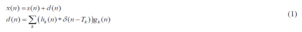
X(n) is the input signal, s(n) is the sum of the clean signal, and d(n) is a noise signal. Tk represents the event time of the kth temporary background noise. The impulse response is defined with hk(n) and the amplitude of the kth noise is denoted with gk(n). An ideal lowpass filter is expressed by the following equations:
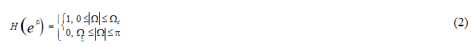
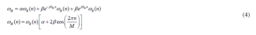
The underwater acoustic signal is a dynamic and non-stationary signal. To solve this problem, the acoustic signals will be converted into small frames by Hamming window. In terms of the rectangular window transform WR(w), Hamming window is shown by the following equations:
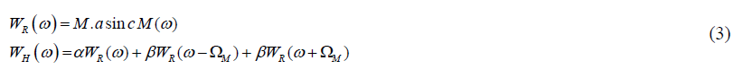
Where M is the window length in samples and αsincM(w) denotes the aliased sinc function. Using the inverse transform of the above equation, the Hamming window is determined by the following equations:
The acoustic data in dataset has a sample rate of 52.734 kHz. Now, these data are re-sampled at 26.367 kHz.
Down sampling a sequence c[n] by a factor D is an operation that retains one out of every D element of c[n], Thus, the output d[n] of a factor-D down sampler is given by the following equation:

A sequence c[n] is passed through a filter h[n] before down sampling by D. The h[n] with a factor-D down sampler is shown by the following equation:

One way to obtain the transformed output from the input is expanding the frequency response of the incoming signal in the range [−π, π] by a factor of D and then creates aliases with spacing π. If the size of each data becomes half of its original size, the generated model will be faster. The chart of the pre-processing stage is shown in Figure 2.

Figure 2: Block diagram of underwater acoustic signal preprocessing.
Spectrogram
To extract the features of acoustic signals based on frequency, it is necessary to divide the signal into its frequency values using the Fourier transform. There is a method for calculating the features of an audio signal that extracts the frequency values along with the time. This visual display of audio signal frequencies over time is called a spectrogram. The Fourier transform is suitable for determining sinusoidal components of a time domain signal x(t). A simple way to overcome the problem of using the fourier transform is to use basis functions to extract features in both the time and frequency domains. Short-Time Fourier Transform or STFT is defined as the following equation:
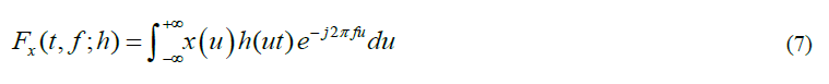
Where h(t) is a short time analysis window localized around t=0 and f=0. The spectrogram is given by the following equation:
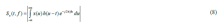
Figure 3 shows spectrogram images related to underwater acoustic signals emitted from 4 classes of ships.

Figure 3: Spectrograms of the acoustic signals emitted from 4 classes of ships.
MobileNet
After the emergence of the AlexNet convolutional network and winning the 2012 ImageNet Large Scale Visual Recognition Challenge (ILSVRC) competition, the use of convolutional neural networks has increased in the domain of computer vision. To use deep neural networks in systems with limited processing power such as small computer systems and mobile phones, the MobileNet neural network with fewer parameters, faster execution speed, and acceptable accuracy was formed. One of the problems of using standard convolution is its high calculations, Therefore, another type of convolution layer called Depthwise Separable (DWS) convolution is used, which requires fewer calculations. Standard convolution in the discrete time domain is given by the following equation:

Where x[n] is input signal, h[n] is impulse response, and y[n] is output. * Denotes convolution. 2D convolution is represented as follows:

Depthwise separable convolution uses two layers called Depthwise Convolution (DW) Pointwise Convolution (PW) to reduce calculations. a k × k kernel is utilized in the depthwise convolution layer and then, the pointwise convolution layer uses m kernel numbers c × 1 × 1 to generate new feature maps. Mathematical calculations of separable Convolution 2D are defined as follows:

The high-cost layers at the beginning and end of the network are redesigned and a new nonlinear function, h-swish, is used instead of the ReLU nonlinear function. Hard swish or h-swish is the non-linear function that improves the accuracy of neural networks which are represented as follows:
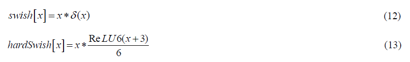
Figure 4 shows the performance of standard convolution and depth separable convolution. In the design of the MobileNet network.

Figure 4: Comparing the processing of traditional convolution and depth wise separable convolution.
The DW convolution filter performs a single convolution on each input channel and the PW convolution filter, combines the DW convolution output linearly with a 1 × 1 kernel, as shown in Figure 5. In the first layer, a standard convolution layer is considered and stride is adjusted in the first layer of convolution by 2. In the next layers, all layers are depthwise separable type convolution [4, 5].

Figure 5: Processing of different layers of mobilenet network in the proposed method.
The filter size of all DW convolution layers is 3 × 3. After that, 2 layers with 32 filters and then a PW convolution layer with 64 filters are considered. Then 9 layers with 128 filters are placed. In the end, there will be 2 layers of 1024 filters. We used the Softmax classifier at the end of the model structure. The model structure is shown in Table 2 and the diagram of the model is shown in Figure 6.
| Type/Stride/Activation | Filter shape | Input size |
|---|---|---|
| Conv 2D/s2/h-swish | 3 × 3 × 3 × 32 | 224 × 224 × 3 |
| Conv dw/s1/ReLU | 3 × 3 × 32 dw | 112 × 112 × 32 |
| Conv pw/s1/ReLU | 1 × 1 × 32 × 64 | 112 × 112 × 32 |
| Conv dw/s2/ReLU | 3 × 3 × 64 dw | 112 × 112 × 64 |
| Conv pw/s1/ReLU | 1 × 1 × 64 × 128 | 56 × 56 × 64 |
| Conv dw/s1/ReLU | 3 × 3 × 128 dw | 56 × 56 × 128 |
| Conv pw/s1/h-swish | 1 × 1 × 128 × 256 | 28 × 28 × 128 |
| Conv dw/s1/h-swish | 3 × 3 × 256 dw | 28 × 28 × 256 |
| Conv pw/s1/h-swish | 1 × 1 × 256 × 512 | 14 × 14 × 256 |
| Conv dw/s1/h-swish | 3 × 3 × 512 dw | 14 × 14 × 256 |
| Conv pw/s1/h-swish | 1 × 1 × 512 × 512 | 14 × 14 × 512 |
| Conv dw/s1/h-swish | 3 × 3 × 512 dw | 14 × 14 × 512 |
| Conv10 pw/s1/h-swish | 1 × 1 × 512 × 1024 | 7 × 7 × 512 |
| Conv11 dw/s2/h-swish | 3 × 3 × 1024 dw | 7 × 7 × 1024 |
| Conv11 pw/s1/h-swish | 1 × 1 × 1024 × 1024 | 7 × 7 × 1024 |
| Avg Pool/s1 | Pool 7 × 7 | 7 × 7 × 1024 |
| FC | 1024 × 5 | 1 × 1 × 1024 |
| Softmax | Classifier | 1 × 1 × 5 |
Table 2: Light-weight modified mobilenet structure used for image classification.

Figure 6: Overall block diagram of the proposed method.
Results and Discussion
Experimental setup
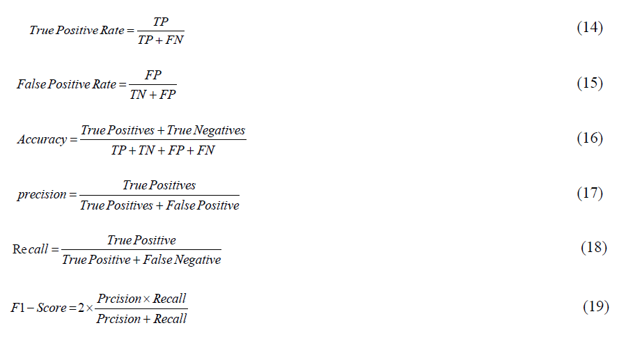
In this research, the data is resampled at 26.367 kHz. Each sample is split into multiple segments to be processed for input to the model’s algorithms. Considering the features of passive sonar audio signals, computing resources, and Classification accuracy, each signal is divided into 4-second segments. The features extracted from the sonar dataset in the time frequency domain are accumulated in the form of spectrogram images. These spectrogram images are utilized as input to the suggested classifier model. By segmenting and calculating the frequency spectrum, many 5671 spectrogram images are obtained in the dimensions of 224 × 224 × 3, which belong to 5 defined classes of types of vessels. 70% of this data was used for training, 20% for validation, and 10% for testing. The evaluation of algorithms is estimated with four parameters (accuracy, precision, recall, and F1-score). The evaluation equations are calculated through the following equations [6].
Using the confusion matrix, the reliability and accuracy of the classification in different classes are determined. In the bottom part of Table 3, the confusion matrix information is shown [7].
| Actual value | True | False | |
|---|---|---|---|
| Predicted value | True | True positive (Correct detection) | False negative (False detection) |
| False | False positive (False alarm) | True negative (Correct detection) |
Table 3: Confusion matrix for image classification.
We train the designed model for training data with 64 batches and 20 or 50 epochs. In this research, four models based on deep learning (standard CNN convolutional network, VGG network, ResNet network, and LeNet) and their popular use in underwater acoustic classification have been selected. The results obtained from the proposed method are compared with these methods [8].
Experimental results
The proposed classifier model was built in Python utilizing a Keras sequential model with a Tensorflow backend and is trained in 20 and 50 epochs with a batch size of 64. The recognition accuracy and validation loss of the model have been obtained for both the training and validation datasets and their results are shown in Figure 7.

Figure 7: Plot of loss and classification accuracy of the proposed model. (a) 50 epochs and (b) 20 epochs.
The results obtained in Figure 7 show that the classification accuracy increases with the increase in the number of epochs. This means that in larger epochs, more accurate and meaningful features are extracted locally, which enables the network to recognize the target with better accuracy. The confusion matrix for the test dataset sample is shown in Figure 8. The diameter of the matrix represents the results of the recall or the true positive rate, which expresses the correct performance of the model based on the accurate classification of different classes of the dataset. As shown in Figure 8, by increasing the number of iterations, the recognition accuracy increased and different classes of the dataset were correctly classified [9].

Figure 8: Confusion matrix for 5 label classification. (a) 50 epochs and (b) 20 epochs.
The comparative chart of the correct recognition of the test data set related to different classes by the Receiver Operator Characteristic (ROC) curve is shown in Figure 9.

Figure 9: The classification evaluation for 5 classes of the target (a) 50 epochs and (b) 20 epochs.
Bach, Vu, and Nguyen after obtaining spectrogram images of the ShipsEar dataset, used them as input in their proposed model. They selected 100 epochs for training the model and obtained different results using the LeNet, VGG, and CNN algorithms. The classification accuracy of LeNet is only 70%, as shown in Figure 10a, the accuracy of VGG is 78%, as shown in Figure 10b, and CNN obtained the classification accuracy of 87%, as shown in Figure 10c. The elapsed time for training of LeNet and CNN models is almost 150 minutes, while that of VGG is 180 minutes. Consequently, their accuracies are lower than the proposed model with a longer training time [10].

Figure 10: The classification accuracy of spectrogram and different algorithms. (a) LeNet (70%), (b) VggNet (78%) and (c) CNN (87%).
The results of acoustic signal recognition accuracy for all methods are given in Table 4. Accornig to results, the proposed model has achieved 97.37% accuracy, which has outperformed the standard CNN, VGG, ResNet, and LeNet, but it is slightly less than the accuracy obtained in Res-DensNet model with 96.79% accuracy. Also, the precision of 98.37%, recall of 99.04%, and F1-score of 98.84% are other results obtained. By analyzing the results acquired in the evaluation criteria, it can be noticed that the proposed method for accurately detecting the targets of surface and subsurface vessels based on the acoustic signals received from them, compared to other standard methods, has a relatively more appropriate and reliable performance in automatic target detection with an increase It speeds up performance and reduces computational complexity [11-15].
| Method | Accuracy | Precision | Recall | F1-Score |
|---|---|---|---|---|
| LeNet | 0.7 | 0.78 | 0.85 | 0.77 |
| CNN | 0.925 | 0.9475 | 0.996 | 0.8765 |
| VGG 19 | 0.9302 | 0.931 | 0.9322 | 0.9284 |
| ResNet | 0.8812 | 0.8708 | 0.9218 | 0.882 |
| Res-DensNet | 0.9679 | 0.9833 | 0.99 | 0.98 |
| Proposed model | 0.9737 | 0.9837 | 0.9904 | 0.9884 |
Table 4: Classification result of different techniques in percentages for target recognition.
Table 5 shows the computational efficiency of the proposed model according to the number of operations and calculation time performed in each epoch and all epochs. Investigating the used algorithms shows that the number of operational parameters of the suggested technique is far more smallish than the models based on CNN, VGG, Residual, and LeNet. This is due to the use of the average-pooling method and the removal of additional pointwise and depth wise convolutions in the end of the proposed algorithm. Regarding the duration of training and validation calculations, the time spent by the suggested approach is less than the other models [16-18].
| Method | Number of parameters (million) | Computation time of each epoch (second) | Computation time of all epochs (minute) |
|---|---|---|---|
| LeNet | 36 mil | 60.5 sec | 75 min |
| CNN | 5.8 mil | 18.5 sec | 21 min |
| VGG 19 | 20.2 mil | 49.5 sec | 62 min |
| ResNet | 23.8 mil | 58.2 sec | 65 min |
| Proposed model | 2.2 mil | 12.6 sec | 18 min |
Table 5: Comparing the number of parameters and the duration of calculations in different deep learning algorithms. The best timing in each column is shown in bold.
Considering the effect of the training epoch in reducing the validation loss and increasing the model recognition accuracy, in this research, different epochs (epoch=20, 50) were used for data training.
The results displayed in Table 6 show that in training with 50 epochs, the classification accuracy has improved and the evaluation loss has decreased [19].
| Method | Num of epochs | Accuracy | Loss |
|---|---|---|---|
| CNN | 20 | 90.45% | 11.5% |
| 50 | 92.5% | 10.4% | |
| VGG 19 | 20 | 91.81% | 9.6% |
| 50 | 93.02% | 8.2% | |
| ResNet | 20 | 88.01% | 12.6% |
| 50 | 88.12% | 10.5% | |
| Proposed model | 20 | 97.13% | 3.2% |
| 50 | 97.37% | 2.1% |
Table 6: Accuracy and loss results of training models in various epochs.
Gradient descent is an optimization method that iteratively updates the weights. If the network is trained for a few epochs, it will result in under fitting the data. This means that the model cannot capture the underlying trends in the data. When the number of epochs is improved, the network reaches an optimal state that achieves the maximum accuracy in the training set. Now, if the number of epochs increases drastically, it leads to overfitting of the data and the generalization of the model to new data not accomplished correctly. This means that the network does not reflect the reality of the data. Therefore, to have the best performance, the number of epochs in network training cannot be determined in advance. This is a hypermeter that needs to be adjusted heuristically. According to the results of Table 6, by increasing the training epoch from 20 to 50, in all models, a relative improvement in training accuracy has been achieved and the validation loss has decreased [20].
In the performance comparison, the results of the classification tests showed that the accuracy of the proposed methods is significantly better than the traditional deep learning techniques for the classification of 5 targets, and the recognition accuracy performance of VGG is marginally better than the MobileNet model. Also, the accuracy of the proposed method for underwater acoustic target recognition compared with other introduced methods in Table 7.
| Input | Methods | Accuracy |
|---|---|---|
| Spectral envelope normalized | Convolutional neural network | 0.904 |
| Wavelet transform (Average power spectral density) | Multilayer Perceptron (MLP) | 0.94 |
| Wavelet packets | CNN+k-nearest neighbor | 0.9264 |
| Synthetic aperture sonar imagery | Deep convolutional neural network | 0.903 |
| Competitive deep-belief networks | Support Vector Machine (SVM) | 0.9089 |
| Spectrum image | DCGAN+S-ResNet | 0.9304 |
| Spectrogram | Multi-Scale Residual Unit (MSRU) | 0.8315 |
| Waveform | Separable convolutional neural network | 0.9091 |
| Low-Frequency Analysis Recording (LOFAR) | Convolutional neural network | 0.9522 |
| Micro-Doppler sonar | Support Vector Machine (SVM) | 0.9852 |
| Fusion features | Resnet-18 | 0.9431 |
| Multi-Window Spectral Analysis (MWSA) | Resnet | 0.9632 |
| Spectrogram | Resnet and densNet | 0.9769 |
| DEMON and LOFAR | Convolutional neural network | 0.94 |
| Time–frequency diagrams | Bidirectional short-term memory (Bi-LSTM) | 0.97 |
| Acoustic spectrograms | Convolutional neural network | 0.969 |
| (Spectrogram) (Proposed method) | VGG19 | 0.9857 |
| (Spectrogram) (Proposed method) | MobileNet | 0.9737 |
Table 7: Omparison of the recognition accuracy of the proposed model and other existing methods.
As shown in the Table 7 above, compared to the existing methods for performing UATR, the proposed models have high classification accuracy, which can increase the processing speed of target recognition and avoid wasting time in model training calculation operations. In addition, in this research, due to the use of the average integration method at the end of the layers of the convolutional algorithms of the proposed model, instead of the fully connected layer, it has been tried to reduce the complexity and increase calculations. Especially in the MobileNet network, due to the removal of additional point and depth convolutions at the end of the algorithm, the duration of training and evaluation calculations spent by the proposed method is less than the classifier models based on the mentioned convolution methods. The evaluation results of the developed model show that the presented model has the necessary efficiency to recognize and classify different classes of ships.
Conclusion
In this research, we presented a new approach for underwater acoustic target recognition, using the deep learning method (MobileNet) with modified mechanisms at the end of the network in the ShipsEar dataset. To use sonar acoustic data in the proposed model, after performing the necessary preprocessing on them, it has converted them into spectrogram images. To speed up the stages of recognition and classification of targets by the proposed model, it has used the designed convolutional network of MobileNet with the least number of parameters. We demonstrated that using this network can simultaneously extract the time and frequency features of the data by producing spectrograms according to the acoustic data emitted from the ships. We trained the classifier and analyzed its generalization using sonar dataset. The classifier demonstrated satisfactory performance in classifying and recognizing target signals with rare false alarms. In performance comparison, the accuracy of the proposed method has remarkably outperformed standard deep learning techniques for the task of 5-target classification and improved calculation speed and validation loss. Considering the classification accuracy of 97.37% in the proposed method, it can be concluded that this method has achieved advanced accuracy. Regarding the performance of the models, it can be seen that with the increase of layers and convolutional parameters, the accuracy of the model improves negligibly, but the speed of model calculations decreases. In this case, we need powerful hardware to train the model. This research has intensively tried to reach a proper trade-off between the accuracy and speed of the networks so that with the relative improvement of the classification accuracy, they have noticeably reduced the number of parameters and the number of calculations. Although in some models, increasing the number of parameters can lead to higher accuracy; it reduces the speed of performance. The proposed models presented in this paper will run on portable devices and mobile phones. The proposed method aided in the Sonar system's acoustic target classification and recognition.
Funding
The authors did not receive support from any organization.
Conflict of Interest
On behalf of all authors, the corresponding author states that there is no conflict of interest.
References
- Hu G, Wang K, Peng Y, Qiu M, Shi J, Liu L. Deep learning methods for underwater target feature extraction and recognition. Comput Intell Neurosci. 2018.
[Crossref] [Google Scholar] [PubMed]
- Satheesh C, Kamal S, Mujeeb A, Supriya MH. Passive Sonar Target Classification Using Deep Generative β-VAE. IEEE Signal Processing Lett. 2021;28:808-812.
- Mohamed AR, Dahl GE, Hinton G. Acoustic modeling using deep belief networks. IEEE Trans Audio Speech Lang Process. 2011;20(1):14-22.
- LeCun Y, Bengio Y, Hinton G. Deep learning. Nature. 2015;521(7553):436-444.
[Crossref] [Google Scholar] [PubMed]
- Gao Y, Chen Y, Wang F, He Y. Recognition method for underwater acoustic target based on DCGAN and DenseNet. In2020 IEEE 5th International Conference on Image, Vision and Computing (ICIVC), Beijing, China 2020 (pp. 215-221). IEEE.
- Ke X, Yuan F, Cheng E. Underwater acoustic target recognition based on supervised feature-separation algorithm. Sensors (Basel). 2018;18(12):4318.
[Crossref] [Google Scholar] [PubMed]
- Franceschini S, Ambrosanio M, Vitale S, Baselice F, Gifuni A, Grassini G, et al. Hand gesture recognition via radar sensors and convolutional neural networks. In2020 IEEE Radar Conference (RadarConf20), Florence, Italy, 2020 (pp. 1-5). IEEE.
- Choo Y, Lee K, Hong W, Byun SH, Yang H. Active underwater target detection using a shallow neural network with spectrogram-based temporal variation features. IEEE J Ocean Eng. 2022.
- Gorman RP, Sejnowski TJ. Learned classification of sonar targets using a massively parallel network. IEEE Trans Acoust Speech Signal Process. 1988;36(7):1135-1140.
- Chin-Hsing C, Jiann-Der L, Ming-Chi L. Classification of underwater signals using wavelet transforms and neural networks. Math Comput Model. 1998;27(2):47-60.
- Azimi-Sadjadi MR, Yao D, Huang Q, Dobeck GJ. Underwater target classification using wavelet packets and neural networks. IEEE Trans Neural Netw. 2000;11(3):784-94.
[Crossref] [Google Scholar] [PubMed]
- Williams DP. Underwater target classification in synthetic aperture sonar imagery using deep convolutional neural networks. In2016 23rd international conference on pattern recognition (ICPR), Cancun, Mexico 2016 (pp. 2497-2502). IEEE.
- Galusha A, Dale J, Keller JM, Zare A. Deep convolutional neural network target classification for underwater synthetic aperture sonar imagery. InDetection and sensing of mines, explosive objects, and obscured targets XXIV, Baltimore, United States. 2019;11012:18-28.
- Yang H, Shen S, Yao X, Sheng M, Wang C. Competitive deep-belief networks for underwater acoustic target recognition. Sensors. 2018;18(4):952.
[Crossref] [Google Scholar] [PubMed]
- Jiang Z, Zhao C, Wang H. Classification of underwater target based on S-ResNet and modified DCGAN models. Sensors. 2022;22(6):2293.
[Crossref] [Google Scholar] [PubMed]
- Tian SZ, Chen DB, Fu Y, Zhou JL. Joint learning model for underwater acoustic target recognition. Knowledge-Based Systems. 2023;260:110119.
- Hu G, Wang K, Liu L. Underwater acoustic target recognition based on depthwise separable convolution neural networks. Sensors. 2021; 21(4):1429.
[Crossref] [Google Scholar] [PubMed]
- Chen J, Han B, Ma X, Zhang J. Underwater target recognition based on multi-decision lofar spectrum enhancement: A deep-learning approach. Future Internet. 2021;13(10):265.
- Saffari A, Zahiri SH, Khishe M. Automatic recognition of sonar targets using feature selection in micro-Doppler signature. Def Technol. 2023;20:58-71.
- Hong F, Liu C, Guo L, Chen F, Feng H. Underwater acoustic target recognition with resnet18 on shipsear dataset. In2021 IEEE 4th International Conference on Electronics Technology (ICET), Chengdu, China 2021 (pp. 1240-1244). IEEE.
Citation: Akbarian H, Sedaaghi MH (2025) Underwater Acoustic Target Recognition in Passive Sonar Using Spectrogram and Modified MobileNet Network Classifier. Int J Swarm Evol Comput. 14:414.
Copyright: © 2025 Akbarian H, et al. This is an open-access article distributed under the terms of the Creative Commons Attribution License, which permits unrestricted use, distribution, and reproduction in any medium, provided the original author and source are credited.