


Indexed In
- Genamics JournalSeek
- RefSeek
- Hamdard University
- EBSCO A-Z
- OCLC- WorldCat
- Publons
- Euro Pub
- Google Scholar
Useful Links
Share This Page
Journal Flyer

Open Access Journals
- Agri and Aquaculture
- Biochemistry
- Bioinformatics & Systems Biology
- Business & Management
- Chemistry
- Clinical Sciences
- Engineering
- Food & Nutrition
- General Science
- Genetics & Molecular Biology
- Immunology & Microbiology
- Medical Sciences
- Neuroscience & Psychology
- Nursing & Health Care
- Pharmaceutical Sciences
Research - (2025) Volume 14, Issue 1
Stochastic Chaotic Network Vector Fields
Carlos Pedro Gonçalves*Received: 22-Jan-2025, Manuscript No. SIEC-25-28375; Editor assigned: 23-Jan-2025, Pre QC No. SIEC-25-28375 (PQ); Reviewed: 10-Feb-2025, QC No. SIEC-25-28375; Revised: 17-Feb-2025, Manuscript No. SIEC-25-28375 (R); Published: 24-Feb-2025, DOI: 10.35248/2090-4908.25.14.393.
Abstract
The present work addresses stochastic chaotic dynamics in network vector fields described by coupled stochastic differential equations, expanding on stochastic chaos in coupled map lattices. We study the example of a network with local coupling and ring topology with the vector field dynamics at each node being described by locally coupled stochastic differential equations given by the stochastic Lorenz system, the resulting local dynamics, mean field dynamics and synchronization
patterns are researched for different coupling strengths and network sizes, showing the presence of a relation to the Lorenz chaotic attractor as well as multifractal scaling in the field dynamics and multifractal phase transitions. The relevance of the results for the research on the synergetics of complex systems and networked computation is addressed.
Keywords
Stochastic chaos; Network Vector Field Theory (NVFT); Synergetics; Complexity; Computational Field Theory (CFT)
Introduction
Chaos in high-dimensional systems has been subject of research within the context of coupled nonlinear maps [1-5]. These models stand at the intersection between computer science, network science and nonlinear dynamics and are of particular relevance not only in the modeling of turbulence, coevolutionary dynamics, social and economic dynamics but also for dealing with computing systems that involve computing with non-binary values, including analog computation and machine learning models operating on real numbers [1,2,5,6].
The Coupled Map Lattices (CMLs) were among the first such models studied within chaos theory, expanding on the cellular automata discrete state framework to a continuous state computation [1- 6]. High-dimensional chaos, spatiotemporal intermittence and synchronization in nonlinearly interacting networks have been studied in detail in these models as reviewed in [1].
From a mathematical standpoint, we can look at cellular automata, CMLs and other dynamical (computing) network models that have been studied within complexity research, computer science and chaos theory as examples of scalar fields in networks. In the case of cellular automata, these scalar fields’ dynamics can be described by binary values or assume other values in a discrete set of numbers with the real-valued case corresponding to continuous state cellular automata and to the CML models [1,6].
Scalar fields in networks are such that each node in the network is characterized by a number as a computational output from the field’s computation and this number changes in accordance with a local computational rule based upon the network’s connections. This leads to a theory of network scalar field computation.
Indeed, from a systemic standpoint, a network scalar field is associated with a systemic dynamics where the field at each node in the network is characterized by an activity with a computational output that can be addressed mathematically on a numerical scale, in this sense, the field’s activity at each node has a numerical expression and can be addressed in terms of the computational rules leading to local changes in the numeric value (the scalar value) associated with each node in the network.
This type of computational model can be applied to different systems, including number of visits to a network of websites, airport traffic, malware propagation in networks, as just a few examples. Whenever we have a network and a characterization of each node in the network by dynamical scalar data then we can address the problem in terms of a network scalar field model.
Now, one can go beyond the scalar field model and work with vector fields. The difference in this case is that the field at each node in the network has a computational activity that is characterized by a d-dimensional vector as a computational output. This means that the field’s activity at each node has a geometric expression as a vector.
Thus, for a network with n elements we have n × d degrees of freedom related to the field’s computational activity, with d corresponding to the number of field vector components. In the deterministic context, such a computation can either be addressed in terms of a mathematical model as involving a discrete time update rule, or it can be addressed as a flow, in the last case we have a large system of coupled differential equations for the field’s dynamics.
When dealing with chaotic dynamics in this context, we are led to an expansion of the theory of chaos in spatially extended systems, a theory that has been strongly developed in coupled nonlinear maps as reviewed in [1], but that can be expanded to network vector fields characterized by coupled differential equations rather than by coupled maps.
In this context, there is a continuous dynamics of the field at each node, a dynamics that depends upon the network’s connections, leading to continuously changing geometric transformations of the vector at each node in terms of both magnitude and direction.
Now, such as we can transition from a deterministic map to a stochastic map in the context of a coupled map models [1-3], We can also transition from the coupled deterministic flow of the network vector field to stochastic field dynamics.
In regards to the mathematical modeling, the difference is that instead of working with deterministic differential field equations we work with stochastic differential field equations. From a systems’ dynamics standpoint this means that we have an open network’s dynamics with the network field’s dynamics being such that the field computation depends both upon the local nearest neighbours’ field configuration and upon external stochastic environmental fluctuations leading to an external noise source.
In the context of a network vector field characterized by chaotic dynamics this leads to stochastic chaos in network vector fields, characterized by nonlinear stochastic differential equations. The study of such systems is particularly relevant in the context of the synergetic of complex networks as well as for networked computation with real numbers [7-9].
In the current work, we analyze a vector field on a ring network with the field vector components updated in accordance with coupled stochastic Lorenz equations characterized by additive Wiener noise, we study both the local and collective dynamics of such a system, for different network sizes and coupling strengths.
In section 2, we review the main methods, including numeric integration methods and the field equations. In section 3, we study the example network field dynamics characterized by the coupled Lorenz system in a ring network and, in section 4, we conclude with a final reflection on the work’s main results in the context of complexity research, computational field theory and synergetic.
Materials and Methods
Stochastic chaos in nonlinear dynamics can be worked in two settings, stochastic nonlinear maps, which is a discrete time approach and stochastic differential equations (SDEs), in both cases, the main point is that, if we “turn off” the noise process, the corresponding nonlinear deterministic dynamics can be chaotic, that is, bounded, nonperiodic with sensitive dependence upon initial conditions showing random trajectories. In the case of systems described by stochastic differential equations, this means that when the noise process is “turned off” the corresponding system of equations is a standard deterministic system of differential equations.
The main issue regarding chaotic dynamical systems that have a dynamics described by systems of nonlinear differential equations is that their study requires numeric integration. This also means that their stochastic counterparts also require such numeric integration.
The main integration method that we use in the present work is Roberts’ method for numeric integration which is a modified Runge-Kutta method that can be used both for Itô integrals and for Stratonovich integrals [10]. To understand this method, we begin by considering the standard one-dimensional SDE.
As a notation point, we use here capital letters for matrices and vectors and small caps for scalars. In this way, the standard onedimensional SDE used in Itô stochastic calculus can be written as [10]:
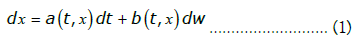
In the above general equation, a is a drift function and b affects the standard-deviation, both are addressed as smooth functions of the argument, dw corresponds to the infinitesimal increments of a Wiener process [10].
The Itô integral is formally addressed by the integration scheme for
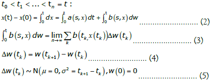
The increments in equation (4) are independent and, as per equation (5), follow a zero mean Gaussian distribution with variance given by  In this way, we have Gaussian IID noise.
The above is the formal basis for stochastic calculus in onedimensional systems, that is, systems with a stochastic scalar variable that depends upon the Wiener innovation, leading to basic processes that are related to one-dimensional Brownian motion. While formal solutions can be built, the basic issue when a and b are not constant is that we may need to employ numeric integration, we follow the modified Runge-Kutta method introduced in [10] for the Itô calculus approximation, which sets Δtk = h and defines the following integration algorithm:
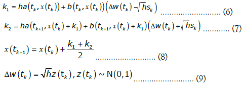
With sk = ±1 with 1/2 probability. In the type of problems that we will be working on, the function b is a fixed scalar which means that we have the basic scheme:
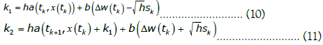
Given these last two equations, applying equation (8), we get the simplified scheme:

Now, the extension to a multidimensional stochastic process requires some care. In our applications, the basic process is given by the vector SDE working with d dimensional vectors:

Where  the Wiener process W is an d-dimensional stochastic vector such that the increments
 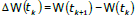 are IID with a multivariate normal distribution with null vector mean, a rank d diagonal covariance matrix with diagonal equal to the numeric integration time step h and W(0) is the null vector. In this case, equations (10) to (12) lead to the vector numeric integration process addressed in [10]:
With Sk being a d-dimensional vector with entries +1 or -1 each selected independently with probability 1/2, of course, since, in our case, b is a fixed scalar, the sum in equation (16) leads to the part dependent upon Sk becoming a null vector not really having impact on the numeric integration.
If b is equal to 0, the above equations lead to a Runge-Kutta method of integration of deterministic differential equations, by contrast if a is constant and b is fixed and different from 0, we get a basic Brownian motion numeric integration scheme with drift parameter a.
In Figure 1, we show the simulation where the equations for a correspond to the Lorenz system in the chaotic phase [11], in the figure, we show the Lorenz chaotic attractor taking b equal to 0 (left), which provides for the deterministic dynamics and taking b equal to 2 (middle) and 3 (right) which correspond to stochastic Lorenz dynamics. As can be seen from the example, when b is set to 0 we get the standard Lorenz chaotic attractor, as b is raised the attractor shape is still present however there is a random motion in the attractor which comes from the additive stochastic component.
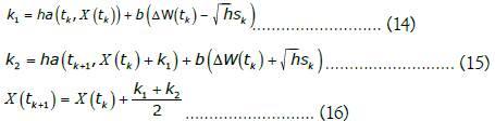
Working from equation (13), the main equations, in vector format using column matrix representation, are given by:
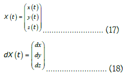
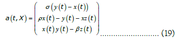
Replacing on equation (13) we can write explicitly the stochastic Lorenz SDE in vector format, in the equation below we omit the explicit temporal dependence for simplification:
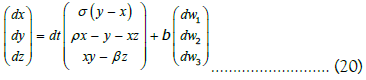
When b=0, we get the deterministic Lorenz equations, which, for the parameters in figure 1, as stated, lead to a chaotic dynamic with the strange attractor structure comprised of two spirals [11,12]. The dynamics is smooth, but nonperiodic, bounded to the attractor and with sensitive dependence upon initial conditions. The topological process that leads to chaos, in this case, is linked to a stretching splitting and merging process [11,12], the final attractor has a fractal structure in three-dimensional Euclidean space, thus, the trajectories follow the fractal geometric structure.

Figure 1: Simulation of the stochastic SDE with a following the Lorenz equations, b=0 (left), 2 (middle) and 3 (right), X(0)=(3,1,1.5), 200,000 steps of 0.001 size are plotted after the first 10,000 were dropped for transients σ=10, ρ=28, β=2.667.
When stochastic coupling is introduced, with additive noise, the displacement in the state vector leads to a stochastic walk on the attractor, as can be seen in figure 1 for b equal to 2 and 3. Thus, the attractor continues to lead the dominant dynamics as a geometric order parameter, however, the noise coupling leads to a nowhere differentiable trajectory on the attractor, contrasting with the smooth differentiable curves that are present in the deterministic case.
While these results are associated with stochastic chaos with a coupling of a low-dimensional nonlinear deterministic system to an additive noise source, we will be dealing here with highdimensional nonlinear dynamics in networked systems, in this way, the deterministic component is high-dimensional and the main equations need to be reviewed for this context, namely, it implies the transition to field equations.
As reviewed in the previous section, such systems have been object of research in the context of coupled deterministic and stochastic maps [1-5], with CMLs being one of the major examples [1]. As reviewed in the introduction, these maps actually deal with scalar fields in networks updated in accordance with a nonlinear rule that depends upon the neighbourhood coupling.
In the present work, we go beyond the scalar field model and expand it to deal with a vector field on the network, which means that the field’s computational dynamics at each node can be described by a vector.
In this way, given the node set  , we deal with an undirected graph described by an adjacency matrix A , where Anm=1 if there is an arc connecting the nodes n and m and 0 otherwise. The network vector field dynamics is formally addressed by a mapping:
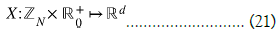
In the above equation, ![]() corresponds to the time coordinate, thus, at each node n and time t, X maps to a d dimensional real vector:
corresponds to the time coordinate, thus, at each node n and time t, X maps to a d dimensional real vector:
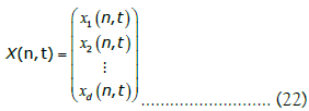
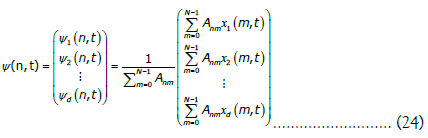
Given the above definitions, the network field dynamical configuration matrix can be written as:
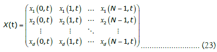
Each column of this matrix coincides with the field vector at a specific node, while each row corresponds to a component of the field vector along the full network. Now, using the adjacency matrix we can extract the local mean field vector for each node as:
That is, we have the local mean field value for each component resulting from the weighted sum of connections of each node with its neighbours, with equal weights, the normalizing factor here is the degree of the node. Considering a local weighted average associated with the local mean field coupling, we get an extension to the continuous time context from the basic scheme used in coupled maps [1], thus, the main SDE is now a field equation of the form:

The stochastic vector dW has a diagonal covariance matrix and is IID for each node, which means that there is no correlation between the additive noise source at each node and also for each vector component. That said, the deterministic part introduced by the drift vector as per field equation (26), by including local mean field coupling, will incorporate both the deterministic and stochastic fluctuations by way of the local mean field coupling, in this case, the drift field vector has a local mean field coupling that is akin to the CMLs’ local mean field coupling using a weighted average model, which introduces a diffusive pattern of coupling [1].
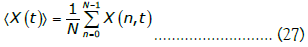
The approach based on the analysis of the global mean field dynamics has been employed in CMLs of one-dimensional nonlinear maps as a way to research these networks’ collective dynamics [1], in this context, the mean field value is a scalar, for a vector field, as per equation (27), that value is a vector with the same number of components as the field vector described in equation (22), therefore, using equation (27), we can implement a d-dimensional representation of the mean field dynamics in Euclidean space to study the mean collective dynamics.
Likewise, we can also represent in d-dimensional Euclidean space the dynamics of the vector field for each node. For up to three-dimensional vectors, this approach provides for a visual representation, in which we plot each column of the matrix in equation (23), which corresponds to each field vector value X(n, t), in a Euclidean space with dimensionality equal to the number of components of the vectors X(n, t). It turns out that, in the case of two or three-dimensional space, this visual representation for both X(n, t) and ⟨X (t )⟩ provides for a relevant visual picture on the geometry of the field’s dynamics, as we will see in the next section.
In the present work, f is given by the Lorenz equations, so that we get the following local field equation SDE, where we omitted the temporal index and used the node as subscript index to simplify the notation:
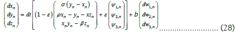
If b is equal to zero, we get a deterministic coupled field dynamics driven by the Lorenz equations with local mean field coupling. Otherwise, we get a stochastic coupled field dynamic.
The stochastic coupling is the difference between a closed network and an open network. In the closed network, the field’s computation at each node has an open dynamic due to the local coupling to its neighbours but the full network is closed, by contrast, in the open network, the field is affected by environmental stochastic fluctuations that affect the field computation at each node.
As stated, due to the local mean field coupling the field’s computation at each node will be affected not only by the stochastic fluctuations at that node but also by the stochastic fluctuations of its nearest neighbours.
From a computational standpoint, we are dealing with networks with nonlinearly interacting nodes affected by external noise, which is a relevant point for current technological frameworks that include machine learning with networked models working on floating point data, with adaptive and possible coevolutionary contexts leading to coevolutionary stochastic dynamics.
A main issue that is raised in this context is the characterization of the collective dynamics depending on both the coupling parameter and the network size. One analysis that is relevant regards the characterization of the scaling of the network mean field vector as given in equation (27).
Indeed, in complex systems, fractal and multifractal scaling is a common occurrence [12,13], the issue then of possible multifractal scaling associated with the network mean field value dynamics is a relevant analysis.
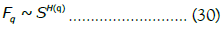
Given a signal u(t), multifractal scaling can be expressed in terms of the moments’ order relation for different lags s [13]:

Thus, the dependence upon the order is given by the product of the order by the generalized Hurst exponent H(q) which can be a nonlinear function of the moment order. One way to estimate the function H(q) is through the application of Multifractal Detrended Fluctuation Analysis (MFDFA) with polynomial fitting, which is a robust method in the detection of monofractal versus multifractal scaling.
The method that we use is described in detail in [14], involving the estimation of a detrended fluctuation function Fq which scales with the lag s as:
This last function is estimated for each component of the network mean field vector, thus, for each component of the network mean field described in equation (27), we apply MFDFA in combination with spectral analysis to characterize the scaling in the network mean field vector components’ dynamics. We also analyse the distribution for the network mean field vector’s displacements in comparison with the multivariate Gaussian distribution, these displacements are given by:
In practice the displacements are, actually, evaluated from the numerical simulation, so that the normality test is applied to the estimated displacements from the simulated trajectory, using a small simulation step, taking the variation of the mean field values as an approximation.
Multifractal processes can include a multifractal Gaussian processes and also non-Gaussian processes [13], while these processes can be directly simulated in a predesigned stochastic process definition, that is, top-down, an approach that is developed in Mandelbrot’s work [13], their occurrence in networked nonlinear dynamical systems may depend upon the interaction profile and system size, in this sense, the approximation to the Gaussian regime or deviations from that regime are the result of the complex nonlinear dynamics and both Gaussian and non-Gaussian dynamics can occur depending upon the network profile and field dynamics.
In this way, we research the profile of the multifractal process and also the distribution profile for different network sizes and local mean field coupling. While different network topologies are possible, we will be working with the one-dimensional lattice model with N nodes and ring topology, where each node is connected to itself and with the left and right node, with periodic conditions at the border, this connectivity structure thus follows the cellular automata scheme [6].
Having presented the main concepts and methods we now address the main results from the simulation of the resulting vector field.
Results and Discussions
In all the simulations that follow we use the network topology addressed in the previous section with one specific point in the adjacency matrix we consider a self-link of each node, therefore, each node is connected to itself and to the left and right neighbors with periodic boundary conditions at the border, leading to the ring-like topology. Given this network structure, the most elementary network is the one with three nodes and periodic boundary conditions. In this case, each node is connected to the remaining two, forming a triangle.
Considering the deterministic dynamics first and the system’s equations formulated in the previous section, we show, in figure 2 top, the plot of the three nodes’ dynamics in the three-dimensional Euclidean space spanned by each of the three components of the field’s vector.

Figure 2: Simulation of three nodes’ ring network deterministic field dynamics for each node (top) and corresponding network mean field (bottom), b=0, σ=10, ρ=28, β=2.667 numerical integration step size 0.01, 50,000 data points shown after the first 10,000 were dropped for transients, initial values selected at random for each node with uniform distribution in the interval [-40,40], with the coupling varying from 0.1 to 0.3 in steps of 0.1.
The plot shows the vector field dynamics without noise at each node with different colors, for local mean field couplings of 0.1, 0.2 and 0.3, respectively, from left to right, the remaining parameters are the ones that lead to the usual Lorenz chaotic attractor [11,12].
As results from Figure 2’s simulation, we find that while the field dynamics at each node, for low coupling, follows the main Lorenz attractor, that is, the field dynamics at each node has the main Lorenz attractor shape as a geometric dynamical order parameter (figure 2, top), due to the low coupling, the field at each node is following different trajectories on the attractor, this leads to a complex network mean field dynamics (figure 2, bottom), which shows two spiraling regions linked to the two spirals of the Lorenz attractor, but there is a more complex dynamics at the center region. This is because the dynamics is not synchronized, due to the low local mean field coupling strength.
As the local mean field coupling strength is increased, the field dynamics still follows the Lorenz geometry, however, the at each node becomes progressively more synchronized with the rest of the network (Figure 3, top), in this way, the network mean field starts to progressively reflect the low dimensional attractor structure (Figure 3, bottom).

Figure 3: Simulation of three nodes’ ring network deterministic field dynamics (top) and corresponding network mean field (bottom), b=0, σ=10, ρ=28, β=2.667, numerical integration step size 0.01, 50,000 data points shown after the first 10,000 were dropped for transients, for the same initial conditions than figure 2, with the coupling varying from 0.4 to 0.7 in steps of 0.1.
For local mean field couplings from 0.5 until 0.6, we, therefore, find that the network (global) mean field reflects the three-dimensional Lorenz attractor, with the field dynamics showing a synchronized trajectory that follows the attractor structure, contrasting with the low coupling case shown in figure 2 bottom and figure 3 in the case of a local coupling of 0.4.
This is an example that fits well a pattern addressed in Haken’s synergetics [7-9], in the sense that the system’s collective dynamics tends to become synchronized with compression in the degrees of freedom, in this case, the full number of degrees of freedom, counted in terms of the number of dynamical variables, is nine, three vector components multiplied by three nodes, but the field dynamics is synchronized leading to a network mean field dynamics that follows the three-dimensional Lorenz chaotic attractor.
Further increasing the local mean field coupling from 0.6 to 0.7 we find, however, that there is a bifurcation in the dynamics going from synchronized chaotic dynamics to a, also synchronized, periodic dynamics with the field dynamics following a closed curve in the geometric space spanned by the field vector components, as can be seen in figure 3, where the 0.7 local mean field coupling value leads to the same curve in both the field dynamics at each node and in the network mean field. In this way, we now have a periodic, rather than chaotic, order parameter characterizing the network field’s dynamics.
This periodic dynamics is unstable in regards to noise, that is, noise can lead it to a new fractal attractor, as shown in Figure 4. Indeed, with low noise, the closed periodic curve becomes the seed to a new fractal attractor that shares some similarities with Lorenz’ attractor but with a few slight differences, namely, a twistor-like shape appears at the center between the two spirals, as shown in Figure 4. The dynamics is still highly synchronized so that the same attractor shape appears in both the field dynamics at each node and in the network mean field, as can be seen in Figure 4.

Figure 4: Simulation of three nodes’ ring network stochastic field dynamics (left) and corresponding network mean field (right) b=0.01, σ=10, ρ=28, β=2.667 numerical integration step size 0.01, network coupling of 0.7, 100,000 data points are shown after the first 10,000 were dropped for transients, initial values selected at random for each node with uniform distribution in the interval (-40,40).
The twistor-like shape is linked to the periodic structure in the noise-free dynamics, the noise, in this case, leads to the strange attractor forming from that seed structure, as can be seen in Figure 5, which superimposes the attractor for the deterministic dynamics and the attractor for the corresponding stochastic dynamics.

Figure 5: Same simulation as in Figure 4, but with added simulation (in black) of the deterministic dynamics obtained for the same initial conditions.
To better visualize the difference with respect to the Lorenz attractor we show, in Figure 6, the projection for the x and y components.

Figure 6: Field components’ x versus y axis projection of three nodes’ ring network mean field dynamics b=0.01, σ=10, ρ=28, β=2.667 numerical integration step size 0.01, network coupling of 0.7, 50,000 data points are shown after the first 10,000 were dropped for transients, initial values selected at random for each node with uniform distribution in the interval (-40,40).
The synchronization dynamics for the network can be evaluated from the dispersion around the network mean field, thus, we can calculate the network standard deviation around the network mean field over time, the higher the standard deviation, the lower the global network synchronization.
The standard deviation, in this case, shows a nontrivial dynamics, that depends upon the network size, indeed, for the stochastic network with noise coupling equal to 0.01 and nearest neighbors’ coupling of 0.7 addressed above, we find that the network mean field and the local field dynamics at each node follow a strange attractor as an order parameter with strong synchronization, however, that synchronization is not static, that is, the field dynamics exhibits fluctuating dispersion, as we will see, this dispersion exhibits multifractal scaling.
Since there are fluctuations in the standard deviation, in Figure 7, we calculate, for different simulations of the network with increasing number of nodes, the mean of the spatial standard deviation around the network mean field, shown in orange, the minimum of that standard deviation, shown in blue, and the maximum of that standard deviation, shown in green, calculated from 100,000 simulation steps, with network sizes ranging from 3 to 200.

Figure 7: Mean (orange), minimum (blue) and maximum (green) of the network standard deviation for each field component around the mean field values for 100,000 simulation steps after the first 10,000 steps were dropped for transients, network sizes ranging from 3 to 200, in steps of 1, b=0.01, σ=10, ρ=28, β=2.667 integration step size 0.01, network coupling of 0.7, initial values selected at random for each node with uniform distribution in the interval (-40,40).
Figure 7’s results show that, for a local mean field coupling of 0.7, noise coupling of 0.01 and low network sizes, the dispersion in the network field values is low, with the minimum, maximum and mean value of the standard deviation of the network field values around the global mean field being close to each other, indicating that, while the dispersion in the field values changes over time, the fluctuations in the standard deviation are low, as are the values of the standard deviation, which indicates a strong synchronization dynamics in each field component.
Thus, in the case of strong coupling for low number of nodes, while the field dynamics exhibits strong synchronization it also exhibits a turbulent dynamic for each field component, with peaks in dispersion occurring around a strongly synchronized dynamics, as shown in Figure 8, for the 3 nodes network.

Figure 8: Network standard deviations for each field component with 100,000 steps, for the three nodes’ network, after the first 10,000 steps were dropped for transients b=0.01, σ=10, ρ=28, β=2.667 integration step size 0.01, network coupling of 0.7, initial values selected at random for each node with uniform distribution in the interval (-40,40).
If the number of nodes is increased, however, we find that, even with local mean field coupling, the field exhibits a sharp rise in dispersion with the interval of variation for the standard deviation rising significantly, as can be seen in Figure 7, this occurs in a way that the maximum dispersion exhibits high values, with the minimum dispersion not increasing significantly with the increase in the number of nodes. In this region, the mean of the standard deviation starts to rise, until it converges to an almost flat line.
The mean of the standard deviation around the mean field tends to stabilize with the increase in network size and the interval of variation for the maximum and minimum start to progressively decrease.
The fact that we have a non-null and, in some cases, even high interval of variation means that the spatial dispersion of the field components around the network mean field fluctuates, which means that there is no fixed spatial distribution, that is, the statistical distribution of the field values in the network is nonstationary with respect to the standard deviation, which is an important finding since it shows that stochastic chaos in network fields, with strong coupling can still exhibit diversity in values, with fluctuating deviations from the network (global) mean field.
In Figure 9, we show the simulation of the network mean field values for each field component, as per equation (27), and the standard deviation around that mean field for a network of 100 nodes, the dynamics seems turbulent both for the mean field and the standard deviation.

Figure 9: Mean field and standard deviation for 100 nodes network, 100,000 steps simulation after the first 10,000 steps were removed for transients, and the remaining parameters the same as those in Figure 8.
The field dynamics at each node still follows the dynamics of the overall Lorenz attractor geometry with its two spirals, as shown in Figure 10, which represents the dynamics of the vector field at each node in the three-dimensional space spanned by the three field components.

Figure 10: Dynamics of the field for the 100 nodes for Figure 9 simulation shown in three-dimensional euclidean space.
Applying multifractal analysis methods to the network mean field dynamics from Figure 10’s simulation, we uncover the presence of multifractal scaling in both the mean field values and in the standard deviation around the mean field, for each field component. The generalized Hurst exponents are all situated above 2, with the highest exponents holding for the negative orders, and the lowest exponents holding for the positive orders, with a descending overall sigmoid curve-like shape holding for both the mean field and the standard deviation dynamics as shown in Figures 11 and 12, for a 100 nodes’ network.

Figure 11: Multifractal spectrum estimation for the network mean field dynamics from Figure 10’s simulation for the x component (left), y component (middle) and z component (right), with 600 lags used and
lags ranging from 1 to 2.5, moments order from -50 to 50, and qn=200.

Figure 12: Multifractal spectrum estimation for the standard deviation around the network mean field values from Figure 11’s simulation for the x component (left), y component (middle) and z component (right),
with 600 lags used and lags ranging from 1 to 2.5, moments order from -50 to 50, and qn=200.

Figure 13: Multifractal spectrum estimation for the network mean field dynamics, with x component (left), y component (middle) and z component (right), and the same parameters as in Figures 11 and 12, but with b equal to 1.
The spectrum shape for the mean field, shown in Figure 11, holds for low noise levels, indeed, as the noise level is increased, there occurs a change in the spectrum shape, corresponding to a multifractal phase transition, with the spectrum leading to a decrease in the exponents and an inversion with the negative orders exhibiting the lower values and the positive orders exhibiting the higher values, as shown in Figure 13.
The multifractal phase transition in the spectrum occurs for all the three field components, as shown in figure 14 (left) for 100 nodes network. However, the shape and changes in the spectrum depend upon the number of nodes in the network, as shown in figure 14 (right) for 3 nodes.

Figure 14: Multifractal spectrum estimation for the network mean field components and same main parameters as in Figures 11 and 12, but with b equal to 0.01, and then from 0.25 to 3, increasing in steps of 0.05, for a 100 nodes network (left) and a 3 nodes network (right).
For noise parameter b values of at least 1, we get a strong stochastic nonlinear dynamic with multifractal scaling for the network mean field. In the strong local mean field coupling regime, this scaling tends to occur with a power law decay in the power spectrum for the network (global) mean field’s vector components, therefore, besides the multifractal signatures we also have 1/f noise signatures in the “spatial” average dynamics, as shown in Figure 15 for a 100 nodes network.

Figure 15: Power spectrum for the network mean field’s vector components (x, left, y middle and z right) in doubly logarithmic scale, for b ranging from 1 to 5 (top to bottom), calculated over 100,000 steps, after the first 10,000 steps were dropped for transients, σ=10, ρ=28, β=2.667, integration step size 0.01, network coupling of 0.7, initial values selected at random for each node with uniform distribution in the interval (-40,40) and 100 nodes.
For a weak network coupling parameter of 0.1, while there is also a power law decay, the decay occurs first faster and then slower for the high frequency spectrum, as shown in figure 16, so that we do not get the large region of straight line decay in the high frequency spectrum as we get in the case with coupling parameter of 0.7, shown in Figure 15.
In the simulations from Figures 15 and 16, we find that the multifractal spectrum for the mean field is such that, for the network strong coupling of 0.7, the lower exponents occur for the negative orders and higher exponents occur for the positive orders, while for the weak coupling of 0.1 we get a reversed spectrum, with the higher exponents for the negative orders and the lower exponents for the positive orders as shown in Figure 17, this exemplifies well how, for different network couplings, multifractal phase transitions can occur.
Figure 15: Power spectrum for the network mean field’s vector components (x, left, y middle and z right) in doubly logarithmic scale, for b ranging from 1 to 5 (top to bottom), calculated over 100,000 steps, after the first 10,000 steps were dropped for transients, σ=10, ρ=28, β=2.667, integration step size 0.01, network coupling of 0.7, initial values selected at random for each node with uniform distribution in the interval (-40,40) and 100 nodes.

Figure 16: Power spectrum for the network mean field’s vector components (x, left, y, middle and z, right) in doubly logarithmic scale, for b ranging from 1 to 5 (top to bottom), calculated over 100,000 steps, after the first 10,000 steps were dropped for transients, σ=10, ρ=28, β=2.667, integration step size 0.01, network coupling of 0.1, initial values selected at random for each node with uniform distribution in the interval (-40,40) and 100 nodes.

Figure 17: Multifractal spectra for Figure 15’s simulations (left) and Figure 16’s simulations (right) 600 lags used with the lags ranging from 1 to 2.5, moments order from -50 to 50, and qn=200.
Another difference between the mean field dynamics regards the statistical distribution for the mean field displacements. Indeed, in the strong coupling regime, for the coupling local mean field coupling parameter equal to 0.7, with high noise, the mean field displacements, approximated as explained in the previous section for the integration step size which in this case is 0.01, tend to follow a Gaussian distribution as shown in table 1, with the Jarque-Bera’s null hypothesis only rejected at 5% and 1% levels for the network mean field displacement vector z component for b equal to 1, and for the network mean field displacement vector y component for b equal to 3 (Table 1).
| b | x component | y component | z component |
|---|---|---|---|
| 1 | 0.8719 | 0.3904 | 0.0058 |
| 2 | 0.8637 | 0.8143 | 0.0748 |
| 3 | 0.5453 | 0.0051 | 0.6655 |
| 4 | 0.7545 | 0.4516 | 0.8865 |
| 5 | 0.8661 | 0.8932 | 0.3644 |
Table 1: Jarque-Bera’s test for normality for the mean field displacement components for Figure 15’s simulations.
As shown in Table 2, for the weak local mean field coupling, deviations from the Gaussian distribution dominate, indeed, for b equal to 1, none of the network mean field displacement vector components have a Gaussian distribution with the p-value of the Jarque-Bera test being equal to 0, as the noise level is increased, the null hypothesis of the test is not rejected at a 5% and 1% levels for the x and y components, however, it is still rejected for the z component [15-18].
| b | x component | y component | z component |
|---|---|---|---|
| 1 | 0 | 0 | 0 |
| 2 | 0.1838 | 0.6877 | 0 |
| 3 | 0.1969 | 0.2175 | 0 |
| 4 | 0.6306 | 0.1629 | 0 |
| 5 | 0.0798 | 0.1305 | 0 |
Table 2: Jarque-Bera’s test for normality for the mean field displacement components for Figure 16’s simulations.
With strong local mean field coupling, Gaussian distribution also tend to dominate for low number of nodes and sufficiently high noise, as shown in table 3 and figure 18, for a local mean field coupling of 0.7.

Figure 18: Multifractal spectra for Table 3, 600 lags used with the lags ranging from 1 to 2.5, moments order from -50 to 50, and qn=200.
| b | x component | y component | z component |
|---|---|---|---|
| 1 | 0 | 0 | 0 |
| 2 | 0.5626 | 0.2042 | 0.0026 |
| 3 | 0.1824 | 0.7362 | 0.4897 |
| 4 | 0.3825 | 0.3927 | 0.17 |
| 5 | 0.7049 | 0.6688 | 0.1913 |
| 6 | 0.9689 | 0.313 | 0.6054 |
| 7 | 0.5185 | 0.9263 | 0.9935 |
| 8 | 0.7135 | 0.0927 | 0.7607 |
Table 3: Jarque-Bera’s test for normality for the mean field displacement components for 3 nodes network, local mean field coupling of 0.7 and the remaining parameters as those of Figure 15.
Decreased local mean field coupling, on the other hand, can lead to a rejection of the Gaussian displacements for the network (global) mean field even with high noise, as shown in Table 4, which shows that for coupling of 0.1, only for the network mean field displacement vector x component does the displacement lead to the non-rejection of Gaussian distribution for sufficiently high noise, however, we still get multifractal spectra.
| b | dx component | dy component | dz component |
|---|---|---|---|
| 1 | 0 | 0 | 0 |
| 2 | 0 | 0 | 0 |
| 3 | 0 | 0 | 0 |
| 4 | 0.006 | 0 | 0 |
| 5 | 0.0459 | 0 | 0 |
| 6 | 0.0611 | 0 | 0 |
| 7 | 0.675 | 0 | 0 |
| 8 | 0.3996 | 0 | 0 |
Table 4: Jarque-Bera’s test for normality for the mean field displacement components for 3 nodes network, local mean field coupling of 0.1 and the remaining parameters as those of Figure 16.
These results show that while multifractal scaling tends to occur in the network’s dynamics the nature of that multifractal scaling, the spectral signal properties of the network mean field and the statistical distribution of that mean field displacement vector depends upon different factors, which include the number of nodes, noise strength and local mean field coupling strength.
Conclusion
The role of stochastic differential equations in computation has been a subject of research within synergetics, computer science and chaos theory with applications including associative memory, complex systems’ dynamics and machine learning.
The dynamics of networked computing systems such as cellular automata and CMLs can, from a mathematical standpoint, be approached in terms of the dynamics of scalar fields in networks, with local field updating based upon nearest neighbors’ connections.
In the present work, we addressed not scalar fields but vector fields in networks with dynamics described by systems of coupled stochastic differential equations, focusing on the example of the stochastic Lorenz equations and a network with ring topology, where each node is connected to the node on the right and left and to itself, with the coupling incorporated in each field component dynamics. The periodic conditions at the borders and the type of network coupling uses the basic cellular automata topology.
From a computer science standpoint, in the context of networked computing systems that operate on real numbers and in a possible continuous time dynamic rather than synchronously iterative scheme, network stochastic vector fields become relevant.
Plotting each network node’s field component dynamics in the three-dimensional space for the field components we find that the field at each node follows the general Lorenz attractor geometry, in this sense, the attractor still works as a geometric order parameter for the network field’s dynamics even for large networks.
On the other hand, for small network size, in this case, for a three nodes’ network, which is the smallest network, we found that, for the deterministic dynamics, as the coupling is increased the dynamics becomes more synchronized with the field at each node and the network mean field following the overall Lorenz attractor structure until, for large enough coupling, a transition to a periodic dynamics occurs, however, this dynamics is highly unstable with respect to noise, adding small noise level an attractor with a different shape is formed with the periodic dynamics’ geometry operating as the seed structure around which the attractor is formed.
We studied the network for different network sizes and coupling, uncovering turbulence in the synchronization dynamics, multifractal scaling in both the network mean field and in the standard deviation around that mean field, multifractal phase transitions, power law scaling in the power spectrum and also Gaussian and non-Gaussian distributions.
The occurrence of multifractal scaling, with local and mean field vector components following an attractor structure, is an important result when dealing with chaos in complex systems with noise, in this sense, the study of network vector field dynamics with equations that exhibit chaotic dynamics and their stochastic counterparts constitutes an important basis on which to research stochastic chaos in complex systems, especially given empirical findings of such dynamics in different systems when employing machine learning for attractor reconstruction.
The research into network scalar and vector fields characterized by stochastic nonlinear dynamics provides for a mathematical basis for the study of the synergetics of networks with complex, possibly stochastic chaotic dynamics, with implications for coevolutionary models of computation. Future research into the dynamics of network scalar and vector fields is needed, with implications for both the theory of hypercomputation in complex systems and the applied research to network dynamics, both natural and artificial.
References
- Kaneko K, Tsuda I. Complex Systems: Chaos and Beyond: Chaos and Beyond: A Constructive Approach with Applications in Life Sciences. Berlin: Springer; 2001: 1-8.
- Gonçalves CP. Financial turbulence, business cycles and intrinsic time in an artificial economy. Algor Fin. 2011;1(2):141-156.
- Losson J, Mackey MC. Evolution of probability densities in stochastic coupled map lattices. Phys Rev E. 1995;52(2):1403-1417.
[Crossref] [Google Scholar] [Pubmed]
- Gupte N, Sharma A, Pradhan GR. Dynamical and statistical behaviour of coupled map lattices. Phys A. 2003;318(1-2):85-91
- Ding J, Lei Y, Xie J, Small M. Chaos synchronization of two coupled map lattice systems using safe reinforcement learning. Chaos, Solitons and Fractals. 2024;186: 115241
- Wolfram S. A New Kind of Science. USA: Wolfram Media;2002
- Haken H. Synergetics – Introduction and Advanced Topics. Berlin: Springer; 2004.
- Haken H. Synergetics and computers. J of Comp and App Math. 1988;22(2-3):197-202
- Haken H. Synergetic computers and cognition: A top-down approach to neural nets. Germany: Springer. 2004: 50.
- Roberts AJ. Modify the Improved Euler scheme to integrate stochastic differential equations. arXiv. 2012: 1210.0933.
- Lorenz, EN. Deterministic nonperiodic flow. J of the Atm Sci. 1963;20(2):130-141.
- Peitgen H-O, Jürgens H, Saupe D. Chaos and Fractals – New Frontiers of Science. Springer;2004.
- Mandelbrot BB. Fractals and Scaling in Finance. Springer: 1997: 13-49.
[Crossref]
- Gorjão LR, Hassana G, Kurths J, Witthauta D. MFDFA: Efficient multifractal detrended fluctuation analysis in python. Comp Phys Commun. 2022;273:108254
- Gonçalves CP. Low dimensional chaotic attractors in daily hospital occupancy from COVID-19 in the USA and Canada. Int J Swarm Evol Comput. 2023;12(1):1000291.
- Gonçalves CP. Chaos-induced self-organized criticality in stock market volatility an application of smart topological data analysis. Int J Swarm Evol Comput. 2023;12(5):331
- Gonçalves CP. Epidemiological rogue waves and chaos-induced multifractal self-organized criticality in COVID-19. Int J Swarm Evol Comput. 2024;13(3):367
- Gonçalves CP. Topological machine learning and chaotic attractors decomposition–an application to sunspot chaos. Int J Swarm Evol Comput. 2024;13:387
Citation: Goncalves CP (2025) Stochastic Chaotic Network Vector Fields. Int J Swarm Evol Comput. 14:393.
Copyright: © 2025 Goncalves CP. This is an open-access article distributed under the terms of the Creative Commons Attribution License, which permits unrestricted use, distribution, and reproduction in any medium, provided the original author and source are credited.