


Indexed In
- Genamics JournalSeek
- RefSeek
- Hamdard University
- EBSCO A-Z
- OCLC- WorldCat
- Publons
- Euro Pub
- Google Scholar
Useful Links
Share This Page
Journal Flyer

Open Access Journals
- Agri and Aquaculture
- Biochemistry
- Bioinformatics & Systems Biology
- Business & Management
- Chemistry
- Clinical Sciences
- Engineering
- Food & Nutrition
- General Science
- Genetics & Molecular Biology
- Immunology & Microbiology
- Medical Sciences
- Neuroscience & Psychology
- Nursing & Health Care
- Pharmaceutical Sciences
Research - (2020) Volume 9, Issue 7
Short-Term Forecasting of Load and Renewable Energy Using Artificial Neural Network
Ram Srinivasan1*, Venki Balasubramanian2 and Buvana Selvaraj32School of Engineering, Information Technology and Physical Sciences, Federation University, Ballarat, Australia
3School of Engineering, Information Technology and Physical Sciences, Federation University, Melbourne, Australia
Received: 25-Nov-2020 Published: 28-Dec-2020, DOI: 10.35248/2090-4908.20.9.192
Abstract
Load forecasting is a technique used for the prediction of electrical load demands in battery management. In general, the aggregated level used for Short-Term Electrical Load Forecasting (STLF) consists of either numerical or non-numerical information collected from multiple sources, which helps in obtaining accurate data and efficient forecasting. However, the aggregated level cannot precisely forecast the validation and testing phases of numerical data, including the real-time measurements of irradiance level (W/m2) and photovoltaic output power (W). Forecasting is also a challenge due to the fluctuations caused by the random usage of appliances in the existing weekly, diurnal, and annual cycle load data. In this study, we have overcome this challenge by using Artificial Neural Network (ANN) methods such as Bayesian Regularization (BR) and Levenberg–Marquardt (LM) algorithms. The STLF achieved by ANN-based methods can improve the forecast accuracy. The overall performance of the BR and LM algorithms were analyzed during the development phases of the ANN. The input layer, hidden layer and output layer used to train and test the ANN together predict the 24-hour electricity demand. The results show that utilizing the LM and BR algorithms delivers a highly efficient architecture for renewable power estimation demand.
Keywords
Forecasting; Accuracy; Short-term load forecasting; Artificial neural network; Wind power; PV power, Electrical load; Aggregated level
Introduction
In the residential areas of Australia, the peak electricity load demand is usually during the afternoons. Surprisingly, the residential afternoon load peak may even be higher than the midday commercial and industrial electricity load demand [1]. To meet such unexpected electricity demands in different sectors and supply the required load, it is necessary to forecast the minimal demand in advance. A Short-Term Load Forecasting (STLF) technique involves collecting data regarding past energy usage and using it to predict near-future loads to meet short-term energy demands [2]. Besides, load forecasting is the strategy used by power-generation companies to predict the charges consumed by a consumer to maintain the power supply–demand ratio.
Accuracy of prediction is a crucial factor that needs to be considered in prediction techniques. However, it is a challenging task requiring significant manual intervention to consider the meteorological factors that affect the predicted results. The accuracy of the forecasting result plays a crucial role in the efficiency of the power supply, and the techniques used for forecasting depend on the forecast period and its purpose. In this work, we performed a detailed analysis of existing short-term load forecasting using Artificial Intelligence (AI) techniques to achieve optimal results for renewable resources such as wind and solar energy. The AI techniques can be divided into the following classes: statistical approach, neural network approach, knowledge-based expert systems approach and hybrid approach, the latter combining one or more approaches. Usually, statistical techniques are used to determine the relationship between weather conditions and the output load of a panel. While Artificial Neural Network (ANN) techniques are generally used to feed the vast collated amount of pre-processed data into the hidden layer for training the network, the advent of powerful computing devices has made it possible to use ANN to train and test data. ANN techniques offer the following benefits:
• Minimization of fault tolerance and flexibility issues
• Increased efficiency due to vast parallelism
• Robustness in handling noisy data
• Real-time prediction
• Ability to achieve a high degree of accuracy of the predicted load.
Background
Load forecasting techniques are the most widely used solutions to meet the demand in power supply. Electricity supplier’s uses past consumption data that can characterize the load forecasting for the estimation of future power utilization to satisfy the future supply and demand [1]. Electricity suppliers face numerous challenges in providing secure, cost-effective and adequate load capacity to the clients in their shelter. The prominent challenges are scheduling, load flow analysis, and planning and controlling the power system. Likewise, there are various aspects that influence forecasting accuracy, such as climate, occasions, celebrations and seasons, which result in varying loads. Accordingly, the utilization of load is predicted by following various ANN techniques.
The three methods incorporated in ANN techniques are short-term, medium-term and long-term forecasting, and they each have appropriate applications. The short-term load forecasting period is generally an hour or a day. The medium-term load-forecasting period is generally a week or even a year. Long-term load forecasting is usually performed over a period of three or four years. The prediction of power utilization is usually carried out yearly in power plants to identify the upper limit of the load.
The motivation behind the forecast is to give the required information to the energy sector that decides and plans the energy requirement with yearly support-plans of intensity in the plant. The fundamental elements influencing medium-term load forecasting originate from factors such as large number of clients, climate conditions, current rebuilding circumstances, national tax approach and others [3].
The factors that influence long-term load forecasting include national financial improvement, populace, mechanical rebuilding and domestic duty arrangement. Generally, the expectation target is the peak load or the month-to-month power utilization in the power plant. The determined information, for the most part, shows repeating values and every long stretch of the year that accompanies the comparable development design [4]. The intention of the forecast is to organize month-to-month upkeep plans, task modes, repository activity plans and coal transportation plans.
STLF is a crucial process, particularly considering the load demand in Australia. During winter, the evening surge in electrical utilization is high in residential areas, while the midday surge will be higher than the evening surge during summer. Therefore, with these fluctuating energy demands, the present need to devise a legitimate energy creation and supply procedure, decrease control wastage and provide sufficient power to the energy grid is of great importance. It is, therefore, increasingly essential to predict future loads on a regular hourly schedule by utilizing short-term electric load forecasting [1]. The short-term load forecasting period is usually every 24 or 48 hours or even fortnightly. The expectation target more often does not depend on the peak energy of an area or the daily or weekly power utilization information [5]. But based on the comparative analysis of the power utilization report for that area, on daily or monthly trends over a year.
The purpose of prediction is to calculate the energy requirement for a day. The fundamental components influencing STLF include week type, climate conditions, electricity tax etc. Conventional methods and neural network-based AI methods are the two kinds of STLF techniques. Nowadays, AI procedures are favored as they are equipped for better performance with nonlinear connections.
Numerous designs have previously been utilized to take care of recurrent issues related to the prediction of the power requirement, which involve methods dependent on direct and nonlinear models [5]. Afterwards, advanced crossbreed models were developed by blending the linear and nonlinear systems. Fuzzy logic method and ANN are two types of AI methods used for performing STLF. However, a significant drawback to the fuzzy logic model is its inability to account for sudden changes in the load [6]. Thus, when there is a load change at a time, it loses its ability to forecast load with required accuracy, resulting in an intolerant error range. Therefore, ANNs are generally preferred to the fuzzy logic method [7].
ANNs stand out amongst the most widely utilized nonlinear STLF strategies. ANN promises the latest systems, which process information and help in detailing a wide range of abilities, which include learning, remembering and generalizing specific patterns and data through training.
There are three layers that form ANN: the input layer, hidden layer and output layer.
ANNs consist of a highly connected array of elementary processors called neurons. ANNs work on the principle of the human nervous system. Information is collected by receptors and fed into the brain as input [8]. The effects convert the feedback in the brain into output through response. In ANNs, a large number of neurons are interconnected in a highly complex, nonlinear and massive parallel network. An ANN with an input layer, one or more hidden layers and one output layer is known as multilayer receptor (MLR) [9]. Each layer consists of several neurons, and each neuron is attached to an adjacent layer with synaptic weights. The training of the neural network minimizes the probable errors, usually a quadratic function of output error.
A network with no hidden layer is called a Single-Layer Neural Network (SLNN). Backpropagation (BP) algorithms are usually applied to single layer as well as multilayer neural networks that as ability to visualize the control images and videos [10].
There is an ongoing debate about devising a more efficient and accurate method to forecast load demand from past consumptions. Many countries have conducted different studies on the model to be used, utilizing multiple variables and integration techniques [11].
There are several additional factors, depending on different regions, that influence the accuracy of the forecasting loads. They include past energy consumptions, Gross Domestic Product (GDP) of the nation, GDP per capita and the population per area. Economic growth of a country, which is GDP per capita, plays a massive role in the bid to meet energy demand. Further, with ever-improving life standards, which are inevitable, energy consumption is expected to steadily increase [12].
Thus, in the literature on energy economics more work was put into obtaining an effective technique to forecast energy demand consumption. There were many methods which came into existence, such as ANNs, fuzzy logic, cross breed and regression models. Among those, the ANNs are the most popular and commonly used forecasting method for obtaining future loads [13]. In this work, the ANN method has been used for achieving STLF. The network has been trained by backpropagation algorithm and results were simulated in MATLAB.
In contemporary lifestyle, the energy demand–supply ratio has to be maintained, for that purpose, high-quality Photo Voltaic (PV) power (or natural power) forecasting is also the need of the hour. In the Photo Voltaic (PV) panels, there are several factors which affect the panel's efficiency. It is important to understand those before moving on to how to forecast PV power for improving productivity. Sunlight is a major factor; however, the factors of wind and temperature affect the efficiency of PV power the most. Wind plays a crucial role in how much energy PV cells can produce effectively [14]. As the heat of the panels increases due to high temperature, the panels provide low energy, thereby decreasing the efficiency of the power generated by the panel, as the temperature is inversely proportional to PV power. Conversely, as the temperature of panels rises, the effectiveness of the PV power falls, and efficiency increases with the cooler panels [15]. In large grid, PV module fault detection is also very crucial [16].
The following section present various strategies utilized for photovoltaic cell, wind and load forecast using neural systems.
Proposed Methodology
The Multi-Layer Perceptron (MLP) of an ANN contains three segments, namely: input layer, hidden layer and output layer. The activation function used in the hidden layer is usually nonlinear (sigmoid or hyperbolic tangent), and the activation function in the output layer can be either nonlinear or linear network. The input layer data has a significant relation to the desired forecast value. Cooling a PV panel by passing wind helps improve the efficiency of PV power. Cooling a PV panel by 1°C, increases its ability to generate PV power by 0.05% based on our simulation.
Further, it is essential to note that this percentage adds up over time. Therefore, before forecasting PV power, it is important to account for natural factors such as wind and temperature and gather, compare and interpret all the essential historical data to obtain processed information on the probability of the logical elements that affects PV power efficiency.
PV System:
Input layer nodes constitute the following components (Figure 1):

Figure 1: The ANN of PV system.
• Temperature
• Irradiance
The above figure depicts the following steps:
• The temperature and irradiance are the inputs considered for the ANN model.
• The network of the hidden layer is feedforward network.
• Training the network using Bayesian method algorithm.
The output of the ANN is to obtain the desired PV power output (in kW).
Wind system
The above figure depicts the following (Figure 2):

Figure 2: The ANN of wind system.
• The temperature is the input considered for the ANN model.
• The network of the hidden layer is feedforward network.
• Training the network using Bayesian method algorithm.
• The output of the ANN is to obtain the desired wind power output (in KW).
Load forecasting
• The inputs considered for the ANN model are the temperature, humidity, an average of 24 hours load (in kW), an average of 168 hours load (in kW) and an average load on weekday, weekend and fortnight (Figure 3).

Figure 3: The ANN of load forecasting.
• The network of the hidden layer is feedforward network.
• Training the network using the Levenberg-Marquardt algorithm.
• The output of the ANN is to obtain the desired overall output load (in kW).
Before collecting data on specified factors, it is crucial to understand the purpose of doing so and to make sure the data corresponding to respective elements is valid.
Since we use photovoltaic cells for electricity, it is essential to interpret the various factors such as temperature and humidity that affect their performance directly or indirectly. If the temperature of the solar cell increases, it rapidly changes the voltage, resulting in a consistent increase in the current, i.e. the net effect is decrease of power in the output with increasing temperature. Due to this, it's crucial to collect historical data of input temperatures, in the unit of degree Celsius, for better and accurate forecasting results.
Another such factor is irradiance. If you consider a photovoltaic cell surface, then irradiance can be defined as the density of solar radiation power received on that surface i.e. (W/M2).
The scope of the load data has an additional impact on the accuracy of the results in that the neurons can be altered to a specific degree, for factor, such as temperature and humidity. The load data with extraordinary values can biasing the outcomes towards the extreme values. The given temperature and load information each get separated by the highest temperature and most extreme load that decrease the prediction accuracy.
As seen in Figure 3, the feed forward network was chosen for the load forecasting as it provides preferred results and the data for the input parameters that are automatically assigned based on the input targets. The hidden layer of the ANN has 16 neurons and a bias model. The bias model’s function is to shift the stimulating function to the right or left because the variation in the data is not enough to reduce the errors to build an efficient forecasting model.
Training the network
The ANN trains the load of wind and PV power. The system learns through precedents, i.e. through system input flags and required outputs. For each information signal, the system creates an output signal, and the learning continues limiting the total of squares of the contrasts between the required and real outputs. From this point, we consider this capacity to be the total of squared errors. The learning is done by feeding repetitive information to the network. One complete presentation of the entire training set is called an epoch. The learning procedure is generally performed on time based on the epoch until the loads balance out and the whole of squared errors combines to a minimum value. The frequently utilized learning calculation for the MLP systems is the Bayesian Regularization algorithm. It is a system for executing gradient descent strategy in the weight space; the slope of the total of squared errors to the individual loads is approximated by reverse-propagating the error signals in the system. The dominant calculation is acquired by utilizing an estimate of Newton’s technique called the Levenberg–Marquardt algorithm. The Bayesian Regularization matrix represents the Jacobian of the minimized function to produce the MLP system. The steps involved in the algorithm are given in Figure 4.

Figure 4: Algorithm for ANN.
• Input Variable Selection: Different variables, which include electric load, type of the day, temperature and spot prices of the past day, and kind of the day, temperature and spot prices of the present forecasting day, are chosen as inputs.
• Data Pre-processing: Incorrect recording of data and observation mistakes are bound to happen. Therefore, abnormal data is interpreted and removed or modified using a statistical method to make sure that the model's continuity is not disrupted (Figure 4).
• Scaling: Considering that the variables fall within vast ranges, the direct usage of network data might incur convergence problems. Multiple scaling schemes are adopted for comparing amongst them and choosing the most suitable one for the forecasting model.
• Training: Each of the three layers’ load and biases are considered when the neural network is initialized. The system modifies the connection strength within the internal network nodes until the proper transformation, which links previous inputs and outputs from the training criteria, is learned.
• Simulation: The trained neural network is used for simulating the forecast output based on the recurring pattern of the inputs given.
• Post-processing: The output obtained from the trained neural network requires de-scaling to generate the desired forecasted loads. If needed, special events can be taken into account at this stage.
• Error analysis: As characteristics of the load change, error observations are essential and should be concentrated on more for better forecasting process by using the Levenberg– Marquardt and Bayesian Regularization methods.
The merits of load forecasting is it can train a large amount of data and the output performance depends upon the trained parameters and dataset relevant to training. While the demerits are to determine a proper network structure and the difficulty of problem showing through the network.
Load forecasting
The ANN technique involves the use of following two variables to identify the input data:
• The historical load demand for the year (2013-2014).
• The data acquired in two weeks (measured for 360-hour load).
The input load data is used to train the network as per the Levenberg–Marquardt algorithm iteratively to execute the prediction of load data [17-20].
The input data signals, and desired outputs learned through the historical data is added to the given neural network. For each input data signal, an output signal was produced, which was tested to minimize the sum of squares in the desired output and the actual outputs from the given load. The input–output patterns to the network were carried out by repeatedly feeding training patterns. The learning process was performed based on the epoch until the sum of squared errors was stable—the ANN trained the network with eight inputs to one target, which was the load. The load forecast for the previous day, provided by the input data, corresponded to that of the following day; when compared, the predicted load was close to the actual load, with minimal error. The trained network of the regression plot was found to be 0.9596. The mean absolute percentage load error was 30% and 8.9% for the current day and the forecasted day (the following day) respectively (Figures 5-8).

Figure 5: Measured (actual) 360 hours'’ loads.

Figure 6: Measured (actual vs. predicted load) 360 hours loads.

Figure 7: Regression.

Figure 8: Best validation performance.
Photovoltaic and wind speed
Forecasting is carried out to obtain PV-specific data to add to the input layer. The solar irradiance, temperature and wind speed data play crucial roles in PV power forecasting. To obtain PV power for a specific date, the information, i.e. the output power of the PV module during the previous months, is taken into consideration with a frequency, say one hour. Considering the power is generated only during the day by the PV module, our primary focus in this work was to demonstrate how temperature could affect the output power of PV module, as the temperature during the daytime is mostly high (Table 1). Thus, proper integration of relation between the inputs and the output PV power was crucial. Solar irradiance is measured in terms of (T), ambient temperature as (Ta) and wind speed as (W). The below Table 1 depicts a comparison between the PV and wind power values (Figures 9 and 10).
| Period | PV | Wind Power |
|---|---|---|
| MSE | 0.0889 | 3e-5 |
| Epoch | 3000 | 10 |
| Time | 16 m.25s | 0s |
Table 1: comparison between wind and pv power.

Figure 9: Wind power.

Figure 10: Wind power (actual power vs. predicted power).
Further interpretation of this data is required for short-term stepwise load forecasting methods to get an articulate PV module temperature and ambient temperature using different input subsets.
The formula for the electric power is

Where,
Radius r= 80 m
Efficiency factor η=40
Air density ρ=1.2 kg/m3
v is the wind speed in km/h
The maximum capacity of the wind panel is 16.3 megawatts and the generated power P is 1.96 W.
Photovoltaic speed
The PV module temperature and ambient temperature are two kinds of temperatures that impact PV power output in different degrees. Based on the mutual information theory, the quantitative correlations between the two temperatures and PV power output are analyzed. In weather classifications, the impact of PV module temperature on the PV power output is more substantial by 20%– 30% than ambient temperature. The solar panels considered for the PV power system in this work, consisting of 10 PV panels of 340 W (Figures 11 and 12).
Total power is 3400 W for 1000((W/m2)).
Input layer: temperature (°C), irradiance ((W/m2)).
Mean squad error

Figure 11: PV power.

Figure 12: PV power (actual vs. predicted power).
Surface temperature plays a crucial role in power generation, while forecasting the Photovoltaic Module the surface temperature affects the efficiency of power generation inversely (Figure 13).

Figure 13: Mean squad error.
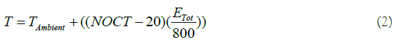
Where,
T represents the PV module’s surface temperature (°C)
TAmbient, represents the ambient temperature (°C)
NOCT, represents the nominal operating cell temperature
ETot represents irradiance level in (W/m2)
The ambient temperature for TAmbient was taken as 25°C with the T=0.82480375 MW.
Results and Discussion
The statistical analysis of prediction of data, in this work, is the combination of Bayesian Regularization and Levenberg–Marquardt algorithm by aggregating numerical or non-numerical information level data collected from multiple sources. PV module temperature and ambient temperature are the two temperature types that impact PV power output in different categories. The performances of ANNs developed by the Bayesian Regularization method using training propagation algorithms in the PV module power estimation were analyzed in this study. The results show that a high-performance level was obtained with the Bayesian Regularization method in PV power estimation at the cost of high computation time. The average mean squad error measured for the output PV power values during the implementation period from 05 May 2019 to 05 May 2020 was 1.96 MW, which reduced to 0.82480375 MW upon using the Bayesian regularization algorithm. This is highlighted by the fact that the proposed photovoltaic power estimation algorithm can be extended to broader PV fleets considerations. The training time for the Bayesian Regularization algorithm was further increased to maintain high accuracy. Consequently, the study shows that the Bayesian Regularization algorithm training results in better performance for ANN-based PV power estimation and when high efficiency is required. The Levenberg–Marquardt algorithm was used to train the data and used to achieve the regression analysis, error measure technique, and mean squad error in this project.
Conclusion
In this study, the Bayesian Regularization method was used for predicting the load, wind power and PV power of panels, a day ahead. The Bayesian approach was determined to be a more suitable choice because of its robustness in sequential data modelling. The obtained predictions are based on non-restrictive hypotheses and can be calibrated and applied to real data. With proper analysis, the wind speed data can be grouped into load forecasts for efficient training and processing; the load data in this study was validated by using real measured data for 2015 and 2019. The results were measured by calculating the error, i.e. the difference between the actual data and predicted information, using performance parameters such as mean squad error and mean absolute error.
REFERENCES
- Wolfs P, Emami K, Lin Y, Palmer E. Load forecasting for diurnal management of community battery systems. MPCE. 2018;6(2):215-222.
- Tsekouras GJ, Hatziargyriou ND, Dialynas EN. An optimized adaptive neural network for annual midterm energy forecasting. IEEE Transactions on Power Systems. 2006;21(1):385-391.
- Saini LM, Soni MK. Artificial neural network based peak load forecasting using Levenberg–Marquardt and quasi-Newton methods. IEE Proceedings-Generation, Transmission and Distribution. 2002;149(5):578-584.
- Orwig KD, Ahlstrom ML, Banunarayanan V, Sharp J, Wilczak JM, Freedman J, et al. Recent trends in variable generation forecasting and its value to the power system. IEEE Transactions on Sustainable Energy. 2014;6(3):924-933.
- Hernández L, Baladrón C, Aguiar JM, Carro B, Sánchez-Esguevillas A, Lloret J. Artificial neural networks for short-term load forecasting in microgrids environment. Energy. 2014;75:252-264.
- Badri A, Ameli Z, Birjandi AM. Application of artificial neural networks and fuzzy logic methods for short term load forecasting. Energy Procedia. 2012;14:1883-1888.
- Chen T, Wang YC. Long-term load forecasting by a collaborative fuzzy-neural approach. Int J Elec Power. 2012;43(1):454-464.
- Banda E, Folly KA. Short Term Load Forecasting Using Artificial Neural Network. Power Tech IEEE Lausanne. 2007;108-112.
- Gezer G, Tuna G, Kogias D, Gulez K, Gungor VC. PI-controlled ANN-based energy consumption forecasting for Smart Grids. 12th International Conference on Informatics in Control, Automation and Robotics (ICINCO). IEEE. 2015;1:110-116.
- Wang Q, Zhou B, Li Z, Ren J. Forecasting of short-term load based on fuzzy clustering and improved BP algorithm. International Conference on Electrical and Control Engineering. IEEE. 2011;4519-4522.
- Hong T, Pinson P, Fan S, Zareipour H, Troccoli A, Hyndman RJ. Probabilistic energy forecasting: Global energy forecasting competition. 2014.
- Webberley A, GAO DW. Study of artificial neural network based short term load forecasting. Power and Energy Society General Meeting (PES). IEEE. 2013;1-4.
- Yang W, Wang J, Wang R. Research and application of a novel hybrid model based on data selection and artificial intelligence algorithm for short term load forecasting. Entropy. 2017;19(2):52.
- Iwashita D, Mori H. Risk quantification for ANN based short-term load forecasting. Electr Eng Jpn. 2009;166(2):54-62.
- Jazayeri K, Jazayeri M, Uysal S. Comparative analysis of Leven berg-Marquardt and Bayesian regularization back propagation algorithms in photovoltaic power estimation using artificial neural network. ICDM. 2016;80-95.
- Mamlook R, Badran O, Abdulhadi E. A fuzzy inference model for short-term load forecasting. Energy Policy. 2009;37(4):1239-1248.
- Hong T, Pinson P, Fan S, Zareipour H, Troccoli A, Hyndman RJ. Probabilistic energy forecasting: Global energy forecasting competition. 2014.
- Sangrody H, Zhou N. An initial study on load forecasting considering economic factors. IEEE (PESGM). IEEE. 2016;1-5.
- Silva LN, Abaide AR, Figueiró IC, Martinuzzi D, Rigodanzo J. Development of an ANN model to multi-region short-term load forecasting based on power demand patterns recognition. IEEE PES ISGT Latin America. 2017;1-6.
- Moon J, Park S, Rho S, Hwang E. A comparative analysis of artificial neural network architectures for building energy consumption forecasting. Int J Distrib Sens N. 2019;15(9):1550147719877616.
Citation: Srinivasan R, Balasubramanian V, Selvaraj B (2020) Short-Term Forecasting of Load and Renewable Energy Using Artificial Neural Network. Int J Swarm Evol Comput 2020; 9:192
Copyright: © 2020 Srinivasan R, et al. This is an open-access article distributed under the terms of the Creative Commons Attribution License, which permits unrestricted use, distribution, and reproduction in any medium, provided the original author and source are credited.