


Indexed In
- Genamics JournalSeek
- RefSeek
- Hamdard University
- EBSCO A-Z
- OCLC- WorldCat
- Publons
- Euro Pub
- Google Scholar
Useful Links
Share This Page
Journal Flyer

Open Access Journals
- Agri and Aquaculture
- Biochemistry
- Bioinformatics & Systems Biology
- Business & Management
- Chemistry
- Clinical Sciences
- Engineering
- Food & Nutrition
- General Science
- Genetics & Molecular Biology
- Immunology & Microbiology
- Medical Sciences
- Neuroscience & Psychology
- Nursing & Health Care
- Pharmaceutical Sciences
Research Article - (2024) Volume 13, Issue 3
Performance Analysis of Backpropagation Artificial Neural Networks with Various Activation Functions and Network Sizes
Hamed Hosseinzadeh*Received: 29-Apr-2024, Manuscript No. SIEC-24-25581; Editor assigned: 01-May-2024, Pre QC No. SIEC-24-25581 (PQ); Reviewed: 16-May-2024, QC No. SIEC-24-25581; Revised: 23-May-2024, Manuscript No. SIEC-24-25581 (R); Published: 31-May-2024, DOI: 10.35248/2090-4908.24.13.368
Abstract
This paper conducts a comprehensive performance analysis of Back Propagation Artificial Neural Networks (BP- ANNs) utilizing various activation functions. Activation functions play a crucial role in shaping neural networks’ behavior and learning capabilities. Through systematic evaluation across diverse network sizes (numbers of hidden layers and neurons), this study assesses the impact of commonly employed activation functions-such as Sigmoidal, Tanh, Clog log, Aranda, and others-on the convergence speed and accuracy of BP-ANNs. The findings provide empirical insights essential for optimizing neural network artificial intelligence architectures tailored to specific applications and datasets.
Keywords
Artificial intelligence; Neural networks; Backpropagation artificial neural networks; Activation function
Introduction
Artificial Neural Networks (ANNs) have emerged as powerful tools for modeling complex relationships and solving intricate problems across various domains. The success and effectiveness of these networks are intricately tied to their ability to learn complex patterns from data. Fundamental to their learning process is the backpropagation algorithm, a cornerstone in training ANNs that adjusts the network’s weights to minimize errors between predicted and actual outputs. ANNs have emerged as powerful tools for complex pattern recognition and modeling across various domains [1]. Besides network size (number of layers and neurons), activation functions are central to the architecture of ANNs. The effectiveness of ANNs heavily relies on their architecture and the choice of activation functions [2,3]. Activation functions introduce non- linearities critical for enabling ANNs to learn intricate relationships within data, thereby significantly influencing their learning capacity [4,5]. Activation functions are pivotal in determining the output of a node or neuron, thereby influencing the network’s capacity for approximation, convergence, and generalization [6,7].
Extensive research has explored the impact of activation functions on neural network performance [8,9]. The study concludes that tanhLU activation functions serve as a superior alternative to traditional tanh functions in neural networks, enhancing performance and accelerating convergence rates across various network types and sizes [10]. Recent advancements have introduced novel activation functions like Swish and Mish aiming to enhance training speed and generalization abilities [11,12]. Different activation functions exhibit unique characteristics; for instance, ReLU and its variants offer faster convergence due to their non- saturating nature while sigmoid and tanh functions face challenges with vanishing gradients [13,14]. However, comprehensive analyses encompassing a broad array of activation functions across diverse datasets remain essential [15-18] and analyses across various architectures and datasets involving these functions remain limited [19].
Although the activation function is a key parameter in a neural network, and the differences between various activation functions are marginal once the network is effectively trained, other factors such as the training algorithm, network size, and learning parameters play a more significant role in the network’s proper training, as evidenced by the minimal differences in training outcomes with different activation functions [20].
Materials and Methods
This paper bridges the gap of performance analysis by systematically evaluating BP-ANNs with a comprehensive set of activation functions across diverse network sizes. This paper enhance evidence and insights that can guide practitioners and researchers in selecting the most suitable activation functions and network size tailored to their problem domains, ultimately enhancing the performance and efficacy of ANNs [21-25].
Simulation method
A code for BP-ANNs is written from scratch in Microsoft Visual Basic 2020. It involves two main phases: the forward pass, where the input data is passed through the network to generate an output, and the backward pass, where the error between the predicted output and the actual output is propagated back through the network to update the weights. This process is repeated for many iterations or epochs (Figure 1).

Figure 1: Schematic diagram of a multilayer perceptron during the back propagation phase, illustrating the flow of error correction from the output layer through the hidden layers to the input layer to adjust the neural network weights.
The general equation for a neuron in an artificial neural network with an activation function can be expressed as:
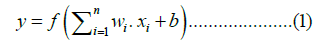
Where y is the neuron’s output, f is the activation function, wi represents the weight of the ith input, xi represents the ith input to the neuron, b is the bias term, and n is the number of inputs to the neuron.
This is the high-level algorithm for BP-ANNs in this research:
Initialization
Initialize weights: Randomly initialize the weights for all layers in the network.
Choose activation functions: Select an activation function for layers (e.g., Sigmoid, Tanh).
Forward pass
For each layer from the input layer to the output layer:
Input calculation: Compute the input to a neuron as the weighted sum of its inputs plus a bias, 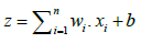
Activation: Apply the activation function to the input to get the neuron’s output, y = f(z)
Backward pass
For each layer from the output layer back to the input layer:
Output error calculation (for the output layer): Calculate the error in the output layer.
Error propagation (for hidden layers): For each layer, calculate each neuron’s delta (error term) based on the deltas of the neurons in the layer above and the derivative of the activation function.
Weight update
For each weight in the network:
Calculate gradient: Compute the gradient of the loss function with respect to each weight. This involves the delta of the neuron it feeds into and the output of the neuron it comes from.
Update weights: Adjust the weights based on the gradients, using a learning rate parameter to control the size of the weight updates.
The overall summary and steps of the above algorithm are:
Forward pass: Compute the output of the network using the current weights and the chosen activation functions.
Calculate total error: Compute the error at the output layer. Depending on the problem, this could mean squared error, cross- entropy loss, etc.
Backward pass: Propagate the error backward through the network, updating weights according to the gradients.
Repeat: Repeat the forward pass, error calculation, and backward pass for many epochs or until the network performance meets a specified criterion.
Results and Discussions
In the investigation of the performance of a neural network model employing the different activation functions (Table 1), the effect of varying the number of hidden layers and the number of neurons in each hidden layer on the model’s accuracy was systematically examined over 1000 iterations. The result in Figure 2 indicates a non-linear (with an oscillation) relationship between the number of hidden layers and the accuracy of the model.
| No. | Name | Function | Range |
|---|---|---|---|
| 1 | Aranda | 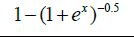 |
[0,1] |
| 2 | Bi_sig_1 | 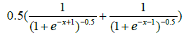 |
[0,1] |
| 3 | Bi_sig_2 | 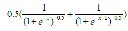 |
[0,1] |
| 4 | Bi_tanh_1 | 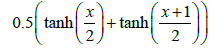 |
[-1,1] |
| 5 | Bi_tanh_2 | 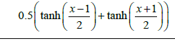 |
[-1,1] |
| 6 | Cloglog | 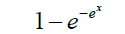 |
[0,1] |
| 7 | Cloglogm | 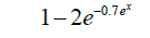 |
[-1,1] |
| 8 | Elliott | 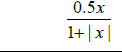 |
[-0.5,0.5] |
| 9 | Loglog | 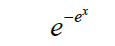 |
[0,1] |
| 10 | Logsigm | 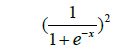 |
[0,1] |
| 11 | Log-sigmoid |  |
[0,1] |
| 12 | Modified Elliott |  |
[-1,1] |
| 13 | Rootsig |  |
[-1,1] |
| 14 | Sigmoidalm |  |
[0,1] |
| 15 | Sigmoidalm2 |  |
[0,1] |
| 16 | Sigt | 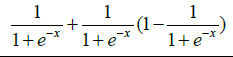 |
[0,1] |
| 17 | Skewed-sig | 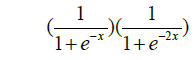 |
[0,1] |
| 18 | Softsign | 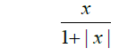 |
[-1,1] |
| 19 | Wave |  |
[- 0.055,1] |
Table 1: Activation functions and their definitions.

Figure 2: Variation of model accuracy with an increasing number of hidden layers in a neural network using the Aranda activation function after 1000 training iterations. The graph exhibits a complex, non-monotonic relationship, with initial high accuracy at a low number of hidden layers, a marked decrease and subsequent minimum at an intermediate number of layers, followed by a steady increase to a plateau like as the number of hidden layers reaches 14000.
The model begins with a high level of accuracy, even with a minimal number of hidden layers, suggesting that the Aranda activation function is highly effective when the complexity of the model is low. As the number of hidden layers increases to 2000, a slight decrease in accuracy is observed, potentially indicating an overfitting scenario where the model is too tailored to the training data, negatively impacting its generalization capabilities.
A significant observation is made as the number of hidden layers’ approaches 4000; the accuracy sharply drops to its lowest point. This trough may indicate a critical threshold beyond which the addition of layers detrimentally affects the model’s ability to learn and generalize. However, past this point, there is a remarkable recovery in accuracy, which steadily increases with the number of hidden layers. At around 8000 hidden layers, the model’s accuracy is closer to its initial value and continues to rise as the number of hidden layers’ approaches 14000.
The 3D plot of Figure 3 visualizes the relationship between the number of neurons, the choice of activation function, and the resulting accuracy of a neural network after 300 iterations of training. Each activation function is represented by a number on the x-axis, and the number of neurons in the network is on the y-axis. The z-axis indicates the accuracy achieved.

Figure 3: 3D representation of neural network accuracy as a function of the number of neurons and activation function type, post 300 training iterations.
From the surface plot (Figure 3), it is evident that there is a complex interaction between the type of activation function used and the number of neurons in determining the accuracy of the neural network. As the number of neurons increases, there is a general trend of increasing accuracy, although the rate of increase varies across different activation functions. Certain activation functions appear to reach near-optimal accuracy with fewer neurons, while others may require a larger number of neurons to achieve comparable performance.
Notably, some activation functions show a sharp increase in accuracy as the number of neurons grows from a lower to a moderate number, after which the increase in accuracy plateaus. This plateauing effect suggests that for these activation functions, there is a saturation point beyond which adding more neurons does not substantially improve accuracy. This can be critical for computational efficiency and avoiding overfitting. It is noteworthy that the accuracy plateaus for most activation functions after a certain number of neurons, which can be interpreted as the point of diminishing returns. This plateau may suggest that beyond a certain network complexity, the additional computational cost of more neurons does not yield a commensurate increase in predictive performance.
The activation functions such as “Modified_Elliott” and “Elliott” display a steep increase in accuracy as the number of neurons grows, particularly in the range from 1 to 10 neurons. This could indicate that these functions are more sensitive to the network’s complexity, benefiting more from a higher number of neurons. In contrast, functions like “Cloglog” and “Cloglogm” maintain a high level of accuracy across all neuron counts, suggesting a robust performance that is less dependent on the number of neurons. This might be indicative of these functions’ ability to capture complex patterns even with a relatively simpler network structure.
Moreover, the varying performance across different activation functions underscores the importance of selecting an appropriate activation function based on the specific requirements of the task and the data. For example, functions with higher accuracy in smaller networks might be preferred in scenarios with computational constraints.
The color-coded accuracy ranges also offer insight into the reliability of predictions. Activation functions that consistently fall within the range of 0.999-1.000 accuracy would be desirable for tasks requiring high precision. Conversely, functions frequently in the range of 0.000-0.995 accuracy might require further investigation or modifications to improve their efficacy.
The investigation into the accuracy of neural network predictions, with respect to the number of neurons and activation functions, has revealed a multi-faceted relationship. The data presented in the bar charts (Figure 4) categorizes the activation functions’ performance after 300 iterations into three accuracy ranges: 0.000- 0.990, 0.990-0.999, and 0.999-1.000, across four neuron quantity scenarios: 2,10,20 and 30 neurons. For configurations with 2 neurons (Figure 4a), most activation functions cluster within the 0.990-0.999 accuracy range, with only ‘Rootsig’ falling below this threshold. Remarkably, ‘Codegem’ stands out with a near-perfect accuracy in the 0.999-1.000 bracket. As the neuron count increases to 10 (Figure 4b), the majority of activation functions maintain their positions within the 0.990-0.999 range, yet ‘Codegem’ retains its superior accuracy, and ‘Wave’ joins it in the highest accuracy bracket.

Figure 4: Comparative analysis of neural network predictive accuracy by activation function and neuron count. The bar charts depict the accuracy
of predictions after 300 iterations across four neuron configurations: 2 neurons (a), 10 neurons (b), 20 neurons (c), and 30 neurons (d). Each
bar represents an activation function, with the color indicating the accuracy range: Solid blue for 0.999-1.000, striped blue for 0.990-0.999, and
solid light blue for 0.000-0.990. The charts illustrate how predictive accuracy varies with the complexity of the network and the type of activation
function used. Note: ( ) 0.000-0.990; (
 ) 0.990-0.999; (
 ) 0.999-1.000.
When the neuron counts rise to 20 (Figure 4c), there is a notable shift with the majority of activation functions, including ‘Aranda’, ‘Wave’, and ‘Codegem’, reaching accuracies in the 0.999-1.000 range. This trend is further pronounced with 30 neurons Z(Figure 4d), where almost all activation functions achieve top-tier accuracy, suggesting a saturation effect where additional neurons do not significantly differentiate the performance of most activation functions.
These observations suggest that while certain activation functions may inherently perform better with a small number of neurons, the benefit of more complex neuron configurations becomes more universal across different functions. However, it is critical to note the exception of ‘Rootsig’, which consistently underperforms across all neuron counts.
The results of Figure 5 show a significant trend where the increase in the number of neurons tends to improve the accuracy rate, up to a certain point, for most activation functions. In particular, the blue to green gradient transition in the graph denotes this trend clearly. As we move from fewer neurons (towards the front of the graph) to more neurons (towards the back), there is a general increase in accuracy, reflected in the change of color from blue to green.

Figure 5: Three-dimensional surface plot depicting the impact of neuron numbers on the accuracy rate of artificial neural networks, highlighting the performance of various activation functions after 300 training iterations.
However, there is a plateau effect observed for all activation functions, where after a certain number of neurons, the improvement in accuracy becomes marginal. This could suggest that the network has reached an optimal complexity for the problem at hand, and further increases in neuron numbers do not contribute to better predictions, which is an important consideration to avoid overfitting and unnecessary computational cost.
Conclusion
This paper presents a comprehensive evaluation of the impact of activation functions on the performance of backpropagation ANNs. The experiment conducted to assess the impact of the number of hidden layers in a neural network with the activation function (i.e., Aranda) on the model’s accuracy yielded insightful findings. The activation function exhibits a high degree of initial effectiveness, with diminishing and increasing (oscillating) returns upon the incremental addition of hidden layers. These results are crucial for the design of neural network architectures, as they highlight the potential for both underfitting and overfitting, depending on the number of hidden layers used. Further research is warranted to explore the underlying mechanisms at higher hidden layers that result in improved model accuracy.
This analysis suggests a significant relationship between the complexity of the neural network, as dictated by neuron count, and the efficacy of the activation function. While certain activation functions may be better suited for networks with fewer neurons, others scale more effectively with increased complexity. The findings provide a valuable framework for the selection of activation functions in neural network design, emphasizing the need to tailor the activation function to both the specific task and the architecture of the model. It is evident that activation functions such as ‘Wave’, ‘Modified_Elliott’, and ‘Aranda’ tend to perform optimally when the number of neurons is increased, consistently achieving accuracies in the highest values as the neuron count approaches 30. In contrast, functions like ‘Rootsig’ and ‘Softsign’ present a lower performance even with a greater number of neurons, with accuracies falling into the lower values in comparison with other activation functions.
With an increase in the number of neurons from 2 to 30, a clear pattern emerges, indicating the impact of neuron quantity on the accuracy of the model after 300 iterations. For configurations with fewer neurons (2 and 10), certain activation functions such as ‘Wave’ and ‘Codegem’ demonstrate a marked increase in accuracy, which is significantly higher than that of other functions. However, as the neuron count increases to 20 and 30, the disparity in accuracy between different activation functions diminishes, leading to a more uniform performance where most activation functions achieve high accuracy. Notably, the ‘Codegem’ function consistently exhibits high accuracy across all neuron configurations, suggesting its robustness and potential suitability for networks with varying complexities. In addition, the number of neurons in a neural network layer is a critical factor for achieving a higher accuracy rate (more neurons, higher accuracy rate). This finding is pivotal for designing efficient neural network architectures, as it emphasizes the importance of balancing network complexity with computational efficiency. Future neural network designs can leverage these insights to optimize their architectures for improved performance in diverse AI applications.
Declarations
Conflict of interest
The authors declare that they have no conflict of interest.
Data Availability Statement
The datasets generated and analyzed during the current study are available from the corresponding author, Hamed Hosseinzadeh, on reasonable request. The data supporting the findings of this study are contained within the manuscript. Any further inquiries regarding the data can be directed to Hamed Hosseinzadeh at Hamed@uwalumni.com
References
- LeCun Y, Bengio Y, Hinton G. Deep learning. Nature. 2015;521(7553):436-444.
- Nair V, Hinton GE. Rectified linear units improve restricted Boltzmann machines. In Proceedings of the 27th International Conference on Machine Learning (ICML-10). 2010:807-814.
- Glorot X, Bordes A, Bengio Y. Deep sparse rectifier neural networks. InProceedings of the fourteenth international conference on artificial intelligence and statistics. 2011:315-323.
- He K, Zhang X, Ren S, Sun J. Delving deep into rectifiers: Surpassing human-level performance on ImageNet classification. InProceedings of the IEEE international conference on computer vision 2015:1026-1034.
- Maas AL, Hannun AY, Ng AY. Rectifier nonlinearities improve neural network acoustic models. InProc. ICML. 2013;30(1):3.
- Sibi P, Jones SA, Siddarth P. Analysis of different activation functions using back propagation neural networks J Theor Appl Inf Technol. 2013;47(3):1264-1268.
- Agostinelli F, Hoffman M, Sadowski P, Baldi P. Learning activation functions to improve deep neural networks. arXiv preprint. 2014.
- Srivastava N, Hinton G, Krizhevsky A, Sutskever I, Salakhutdinov R. Dropout: A simple way to prevent neural networks from overfitting. J Mach Learn Res. 2014;15(1):1929-1958.
- Ertuğrul ÖF. A novel type of activation function in artificial neural networks: Trained activation function. Neural Netw. 2018;99:148-157.
[Crossref] [Google Scholar] [Pubmed]
- Shen SL, Zhang N, Zhou A, Yin ZY. Enhancement of neural networks with an alternative activation function tanhLU. Expert Syst Appl. 2022;199:117181.
- Ramachandran P, Zoph B, Le QV. Searching for activation functions. arXiv preprint. 2017.
- Misra D. Mish: A self-regularized non-monotonic activation function. arXiv preprint. 2019.
- Glorot X, Bengio Y. Understanding the difficulty of training deep feedforward neural networks. InProceedings of the thirteenth international conference on artificial intelligence and statistics. JMLR Workshop and Conference Proceedings. 2010:249-256.
- Ioffe S, Szegedy C. Batch normalization: Accelerating deep network training by reducing internal covariate shift. InInternational conference on machine learning. PMLR. 2015:448-456).
- Clevert DA, Unterthiner T, Hochreiter S. Fast and accurate deep network learning by exponential linear units (elus). arXiv preprint. 2015.
- Singh B, Patel S, Vijayvargiya A, Kumar R. Analyzing the impact of activation functions on the performance of the data-driven gait model. Results Eng. 2023;18:101029.
- Farzad A, Mashayekhi H, Hassanpour H. A comparative performance analysis of different activation functions in LSTM networks for classification. Neural Comput Appl. 2019;31:2507-2521.
- Feng J, Lu S. Performance analysis of various activation functions in artificial neural networks. J Phys Conf Ser. 2019;1237(2):022030.
- Elfwing S, Uchibe E, Doya K. Sigmoid-weighted linear units for neural network function approximation in reinforcement learning. Neural Netw. 2018;107:3-11.
[Crossref] [Google Scholar] [Pubmed]
- Eckle K, Schmidt-Hieber J. A comparison of deep networks with ReLU activation function and linear spline-type methods. Neural Netw. 2019;110:232-242.
[Crossref] [Google Scholar] [Pubmed]
- Gomes GS, Ludermir TB. Optimization of the weights and asymmetric activation function family of neural network for time series forecasting. Expert Syst Appl. 2013;40(16):6438-6446.
- Sodhi SS, Chandra P. Bi-modal derivative activation function for sigmoidal feedforward networks. Neurocomputing. 2014;143:182-196.
- Gomes GS, Ludermir TB, Lima LM. Comparison of new activation functions in neural network for forecasting financial time series. Neural Comput Appl. 2011;20:417-439.
- Singh Y, Chandra P. A class+ 1 sigmoidal activation functions for FFANNs. J Econ Dyn Control. 2003;28(1):183-187.
- Chandra P, Singh Y. A case for the self-adaptation of activation functions in FFANNs. Neurocomputing. 2004;56:447-454.
Citation: Hosseinzadeh H (2024) Performance Analysis of Backpropagation Artificial Neural Networks with Various Activation Functions and Network Sizes. Int J Swarm Evol Comput. 13:368.
Copyright: © 2024 Hosseinzadeh H. This is an open-access article distributed under the terms of the Creative Commons Attribution License, which permits unrestricted use, distribution, and reproduction in any medium, provided the original author and source are credited.