


Indexed In
- CiteFactor
- RefSeek
- Directory of Research Journal Indexing (DRJI)
- Hamdard University
- EBSCO A-Z
- Scholarsteer
- Publons
- Euro Pub
- Google Scholar
Useful Links
Share This Page
Journal Flyer

Open Access Journals
- Agri and Aquaculture
- Biochemistry
- Bioinformatics & Systems Biology
- Business & Management
- Chemistry
- Clinical Sciences
- Engineering
- Food & Nutrition
- General Science
- Genetics & Molecular Biology
- Immunology & Microbiology
- Medical Sciences
- Neuroscience & Psychology
- Nursing & Health Care
- Pharmaceutical Sciences
Research Article - (2023) Volume 11, Issue 6
Determinants of Household Poverty: Analysis of Multidimensional Aspect in Rural and Urban Areas in Amhara Regional State, Ethiopia
Asmamaw Mulusew1*, Mingyong Hong1, Mesfin W/rufaelc2 and Mebratu Kesete22Department of Economics, University of Gondar, Gondar, Ethiopia
Received: 23-Oct-2023, Manuscript No. RPAM-23-23533; Editor assigned: 26-Oct-2023, Pre QC No. RPAM-23-23533 (PQ); Reviewed: 09-Nov-2023, QC No. RPAM-23-23533; Revised: 16-Nov-2023, Manuscript No. RPAM-23-23533 (R); Published: 23-Nov-2023, DOI: 10.35248/2315-7844.23.11.431
Abstract
It would be easier for policymakers to create effective poverty-alleviation policies and programs for multi-deprived poor households if they were aware of the causes and extent of multidimensional household poverty. To that end, the study tried to measure the intensity, acuteness, and factors that can determine households’ multidimensional poverty in rural and urban areas. The study employed a Logit model to analyse the demographic and socio-economic characteristics of poor households. The MPI method was used to define a multidimensional poverty line threshold for the poor and non-poor. The poverty indices were used to analyse the incidence and intensity of multidimensional poverty among households. The findings of the study show that the multidimensional Headcount ratio (H), Intensity (or breadth) of poverty (A), and total Multidimensional Poverty Index (MPI) were found to be 0.47%, 0.43%, and 0.20% in urban areas and 0.81%, 0.48%, and 0.39% in rural areas, respectively, with much higher values for rural households. The results obtained from a binary logistic model indicate that a household’s education level, remittances, and house ownership were found to be negatively correlated with being poor. Besides, in rural areas, household marital status, livestock, and remittances were found to be negatively correlated with being poor. The variables HH size, sex, and total dependency ratio significantly affected HH falling into poverty, while other variables were not significant and rather inconclusive. The major findings of the study reveal that poverty exists severely in the region, especially in rural areas. This finding strongly supports the idea that multidimensional poverty can be improved in the region by focusing on education, stabilising food prices, and creating job opportunities.
Keywords
Poverty; Multidimensional Poverty Line (MPL); Logistic Model; Determinants; Urban; Rural; Amhara Region
Introduction
There is a consensus that poverty is multidimensional. According to Sen, “poverty should be seen in relation to a lack of basic needs or basic capabilities” [1]. Global poverty, which affects 9.2% of the world’s population, is one of the most pressing problems we currently face [2]. According to the World Bank, an individual is considered to be in extreme poverty if their daily income is less than $2.15 [3]. According to the 2014 edition of Credit Suisse’s annual Wealth Report, “the lower half of the global population collectively owns less than 1% of global wealth.” The richest 10%, in contrast, control 87% of the world’s assets, while the top 1% own “almost half of all assets in the world” [4]. In the meantime, more than three billion people, or nearly half of the world’s population, survive on less than $2.50 per day, and more than 80% of people live in nations where income disparities are widening, with the poorest 40% of the world’s population receiving only 5% of global income while the richest 20% receive 75% of it [5]. According to a recent assessment, up to two-thirds of the world’s extremely poor people will reside in fragile, conflict-affected states by 2030, making it clear that without further effort, the world’s poverty targets will not be achieved [6].
Sub-Saharan Africa, as a unique region, draws special attention due to its tragic record of having the highest incidence of poverty. Nine of the top ten nations with the highest rates of poverty will be in sub-Saharan Africa by 2030. Experts have offered numerous explanations for the slow improvement in eradicating poverty in Africa. Factors such as labor market shortages, macro-economic shocks and failures, poor governance, corruption, low economic growth, huge debt burden, environmental degradation, migration, unemployment, underdevelopment, crime and violence and a rapidly growing population, among others, continue to mask the effect of poverty alleviation programs [7]. Although some progress in tackling poverty has been achieved in Sub-Saharan Africa (SSA), there is a wide disparity in the rate of success, since poverty is not experienced in the same manner among the poor and not every nation in SSA has witnessed a steady reduction in poverty.
Ethiopia is the poorest country, and its per capita income is among the lowest of the least-developed countries. In terms of welfare measures, Ethiopia is a desperately poor country. Poverty in Ethiopia is a widespread, multi-faced, longstanding problem that affects a significant portion of its rural and urban population and is measured mainly in terms of food consumption, set at a minimum nutrition requirement. According to the FDRE Planning and Development Commission’s 2021 report, the proportion of people who live below the national poverty threshold has reduced from 44% in 2000 to 19%. 68.7% of Ethiopia’s population is multidimensional poor, while another 18.4% is at risk of falling into this category. Between 2015–2016 and 2019–2020, the poverty rate decreased from 23.5% to 19%. With a Human Development Index of 0.448 and a Multidimensional Poverty Index of 0.564, which gives a rank of 174 out of 188 countries, the nation was identified as one of the poorest in Sub-Saharan Africa. In addition, Ethiopia had one of the highest rates of poverty in the world in 2000, with 44% of the population living below the national poverty level and 56% of the population living below the international poverty line of US$1.25 PPP per day [8]. The national absolute poverty line was set at 7184 Birr per adult equivalent per year in 2016 prices. In rural Ethiopia, 96.3% are poor, while in urban areas, the percentage of poverty is 46.4%. Comparing those two areas, poverty in rural areas was much more severe than in urban areas. In terms of regional poverty rates, Somalia has the highest rate at 93%, followed by Oromia (91.2%) and Afar (90.9%). The Amhara region has a 90.1% poverty rate, while Tigray has an 85.4% rate [9]. For instance, the percentage of people living below the poverty line in rural areas was 25.6%, compared to 14.8% in urban areas [10]. The World Bank noted that the poverty gap index in rural areas was 7.4%, compared to 3.6% in urban areas, and that the severity index for rural poverty was 3.1%, which was marginally higher than the urban poverty severity index (1.4%) [11]. Currently, 23% of Ethiopians live below the national poverty line, which is roughly $2.04 per day, and 27% live below $2.15 [12]. Thus, reducing multidimensional poverty, which is an important determinant variable of economic growth, entails identifying factors that cause poverty. In general, the study tries to identify some major determinants of poverty, the incidence and acuteness of multidimensional poverty, and the characteristics of Poor households in rural and urban areas. Hence, the Ethiopian government has carried out far-reaching institutional and policy reforms to achieve sustainable development, including the Growth and Transformation Plan (GTP). Throughout this time, agriculture has made a significant contribution to value-added. However, over time, the importance of agriculture has fallen (from 52% in 2004 to 37.64% in 2022). High risks in agriculture and limited alternative sources of income result in large fluctuations in individual incomes. Ethiopia’s life expectancy in 2023 was 67.81 years, up 0.55% from 2022 [13]. And Ethiopia’s unemployment rate climbed from 16.90% in 2016 to 19.10% in 2018 [14]. Similarly, 89 million people lack access to clean water; therefore, the difficulties are enormous. More than 75% of the population falls into this category. 90% of kids lack access to even the most basic hygienic facilities [15].
Amhara region, which represents more than 27% of the national population, consists of 10 administrative zones, one special zone, 105 word as, and 78 urban centers, and covers an estimated area of 170,752 square kilometers, of which about 85% of the people are engaged in agriculture, even though the Region is still characterized by the persistence of food shortages, poverty challenges, and the need for better intervention. According to Agegnehu, the proportion of food-insecure households is roughly 42.5% in the Amhara area, which is substantially higher than the national average of 33.6% [16]. Regarding food poverty, the area had the worst score in the nation. The percentage of households experiencing food insecurity is roughly 44.6% in rural areas and 28% in urban areas, respectively [17]. These all suggest that despite the country’s economic growth, food insecurity is a persistent issue in the region.
Taking into consideration these considerations, there are different factors, namely household head size, employment, marital status, age, sex, health, education, remittance, and living standards (cooking fuel, sanitation, water, electricity, floor, and assets), that determine multidimensional poverty in rural and urban areas of the Amhara region. In general, most poverty empirical literature in Ethiopia dominates either rural or urban areas, which are neglected simultaneously in both areas and to the best of the researcher’s knowledge, no published (sufficient) study has been conducted (documented) in the study area dealing with determinants of household multidimensional poverty both in rural and urban areas. Therefore, this study would attempt to measure the intensity, acuteness, and factors that can determine household multidimensional poverty in rural and urban areas in the Amhara region, in addition to coming up with the new international Measure of Poverty (MPI) for the existing problems in this study area.
Literature Review
One of the biggest problems facing humanity is the eradication of poverty in all of its manifestations. The extant literature amicably portrays that poverty is a “multidimensional phenomenon” and should therefore be measured by considering multiple indicators of well-being. According to Alkire, poverty has three dimensions and is made up of ten indicators [18]. The first dimension is health, which has two indicators (nutrition and child mortality); the second dimension is education (indicated by years of schooling and school attendance); and living standards (cooking fuel, sanitization, water, electricity, floor, and assets) make up the last dimension. For example, Achenafi investigated the factors that contribute to urban poverty in Gondar City, Amhara Regional State, Ethiopia [19]. The study made use of original information gained from 220 sample houses through semi-structured questionnaires, focused group discussions, and key informant interviews. It was discovered that the impoverished were more likely to be illiterate and lacked other essential amenities like water and health care. Monthly household income, household size, remittance, metered energy, and household health status significantly impacted the incidence of poverty from the hypothesized variables.
Esubalew researched the factors that contribute to urban poverty in Debre Markos, Amhara Regional State, Ethiopia [20]. A logistic regression model was used in the study, which used primary data from 260 household heads. The primary factors that affect household poverty include sex, household size, disease prevalence in the household, income, educational attainment, marital status, employment, age, tenure of housing, and water supply. The study indicated that 172 (or 66%) of them were considered to be poor, with the headcount, poverty gap, and severity index of the survey coming in at 0.66, 0.21, and 0.09, respectively.
Tesfaye conducted a study on “Determinants of Vulnerability to Poverty in Amhara Regional State, Ethiopia: Evidence from Rural Households of Gubalafto Woreda” [21]. The primary data came from a stratified random sample of 250 houses. The OLS and 3FGLS analytical models were used to determine the future poverty rate for the sampled families, which was determined to be 37.42%. Just 30.8% of the tested households in the study’s early stages were unable to provide for their basic needs. According to the study, factors such as family size, wage employment, proximity to a primary market, and the Kolla agroecological dummy all have a positive effect on a person’s vulnerability to poverty. On the other hand, oxen, land size, non-livestock assets, company ownership, access to financing, and the availability of extension services all significantly and adversely affect vulnerability to poverty.
Anteneh and Daniel conducted a study on “Determinants of Poverty in Rural Ethiopia: Evidence from Tenta Wereda Amhara Regional State,” which was framed by a mixed research design and used a multistage sampling procedure to choose 196 representative samples [22]. The results indicate that 67.3% of societies in the study region live below the national poverty level, which is 387.43 ETB per person per month and 4649.16 ETB per year. A rural household is more likely to overcome poverty if it has beehives, a large farm, oxen and small ruminant animals, and a male head of household. On the other hand, non-farming activity and family size increase the risk of poverty. Therefore, the criteria that determined rural poverty were the sex of the household head, the size of the farmland holding, the number of beehives owned the number of oxen and small ruminants, the size of the household, and non-farm activities.
Desalegn studied “Determinants of Rural Poverty in Banja District of Awi Zone, Amhara Regional State, Ethiopia” using 190 households [23]. Inferential statistics and an econometric model were used to analyze data on the existence and severity of poverty. Therefore, the Cost of Basic Needs method was used to determine the poverty line, which came out to be Birr 4301 per adult equivalent per year. 44% of sample homes were determined to be below the poverty line, while the poverty gap and severity of poverty were, respectively, 9% and 2%, according to the Foster, Greer, and Thorbeck measure of poverty. Thus, it was determined that it took poor households 3.35 years on average to escape poverty. The Tobit model’s results showed that household size had a significant and positive impact on poverty while having a negative impact on it were the number of cattle and oxen owned, the household head’s educational level, the use of inputs, asset ownership, and credit usage in the research area.
Markew and Solomon studied “The determinants of household poverty: the case of Berehet woreda, Amhara regional state, Ethiopia”[24]. Using a stratified simple random selection technique, a sample of 384 homes was selected for the investigation. Foster Greer Thorbecke’s Poverty Index was used to measure the intensity and breadth of poverty in the Woreda. According to their research, 36% of households in Woreda are considered to be below the poverty line, with a 12% average poverty gap and a 7% average severity of poverty. The binary logit model showed that the household dependence ratio, residential location, household education status, and access to credit were all statistically significant in predicting household poverty status.
Eshetu and Gian analyzed “Determinants of farm household poverty status in South Wollo Zone, Amhara Regional State, Ethiopia”, and 516 farm households were included in the study [25]. According to the results of the probit model, family size, dependency ratio, head’s religion, and average distance to various services have positive associations with rural households’ poverty status, educational level, use of irrigation, livestock ownership, participation in non-farm activities, size of farmland, and agro- climate zones have negative associations, The results of the probit model demonstrate that while family size, dependency ratio, the head’s religion, and the average distance to various services have positive associations with rural households’ poverty status, educational status, use of irrigation, livestock ownership, participation in non-farm activities, size of farmland, and agro- climate zones have negative associations.
Tadewos investigated “Magnitude and Determinants of Rural Household Poverty in Ebinat District of Amhara Regional State of Ethiopia”, drawn from 367 households [26]. The results of the logit estimation also indicated that the chance of poverty in a home was positively and significantly influenced by the size of the family and the price of fertilizer. It was observed that the following factors all had a theoretically consistent, statistically significant, and negative impact on poverty: saving culture, land size, livestock holding in TLU, farm and off-farm income per AE, family head’s age, and educational level. With the overall poverty level being 4127.42 Birr per AE per year and the food poverty threshold being 3752.20 Birr, respectively, it was determined that 56.67% of the 367 households that were studied were poor. The FGT poverty index was used to determine the amount and severity of poverty. It is clear that 56.67% of the sample households live below the poverty line thanks to the poverty gap and severity index values of 0.1817 and 0.0835, respectively.
The study “Determinants of Rural Household Poverty across Agro-Ecology in Amhara Regional State, Ethiopia: Evidence from Yilmana Densa Woreda” by Birara examined 328 families. Additionally, the findings revealed that Yilmana Densa woreda had a higher poverty headcount ratio (62.3%), poverty gap (18.9%), and severity (5.8%) rates than the national and regional rates [27]. The model’s findings showed that household poverty was significantly and adversely correlated with factors such as level of education, cost of agricultural inputs, agroecology, ownership of land and livestock, preservation of culture, and area of rented land. However, family size, health, inefficient utilization of the workforce, and poverty in the home all revealed a positive and substantial correlation. Kola’s agriculture has higher poverty headcount ratios, gaps, and severity as compared to Dega and Woina-Dega agriculture.
A study on the “Determinants of Urban Poverty in the Case of Debre Birhan Town” was undertaken by Mulugeta using data from 203 randomly chosen sample families in the Amhara Regional State of Ethiopia [28]. Using Food Energy Intake (FEI), 48 (or %) of the 203 household heads that were questioned were classified as being poor. The binary logit regression model revealed that sex, married status, family size, education, income, health status, housing, and electricity are statistically significant predictors of poverty.
Ermiyas et al. investigated the “Determinants of Rural Poverty in Ethiopia: A Household Level Analysis in the Case of Dejen Woreda, Amhara Regional State, Ethiopia” by using 204 households [29]. Accordingly, almost 49% of the examined rural households live below the poverty line, with an average poverty gap of 0.083 and a poverty severity gap of 0.065. The probit model was used to explore the primary drivers of rural poverty. The probit model study’s findings show that household size, sex composition, dependence ratio, and livestock ownership are the primary determinants driving rural poverty. Poverty status is inversely correlated with the total number of animals a household owns and the gender of the household leaders (male dummies). On the one hand, there is a positive correlation between family size, the proportion of dependents, and household poverty.
Methodology
Source of data
The only secondary data source used in this analysis was the Ethiopian Socioeconomic Survey (ESS), a joint effort of the World Bank’s Living Standards Measurement Analysis-Integrated Surveys of Agriculture (LSMS-ISA) project in 2013/2014 and the Central Statistics Agency of Ethiopia (CSA). Quantitative and qualitative information about the social, demographic, and economic characteristics of households was acquired through surveys [30] (Table 1).
| Data description | Proxy | Sources |
|---|---|---|
| HH head age | Household head age | World Bank ESS |
| Sex of HH | Household head sex | World Bank ESS |
| HH size | Household family size | World Bank ESS |
| House owned | Household house ownership | World Bank ESS |
| Marital status | Household head marital status | World Bank ESS |
| Employment status of HH | Household employment type | World Bank ESS |
| HH head education | Household head education | World Bank ESS |
| Remittance | Remittance | World Bank ESS |
| Access to off-farm income | Access to off-farm income (households with off-farm income) | World Bank ESS |
| Total dependency | Dependency ratio | World Bank ESS |
Table 1: Data source and data description.
Methods of data analysis and estimation techniques
To realize the objectives of the study, the researcher constructed the multidimensional poverty index (MPI), followed by an identification of indicators to identify the direction and significant determinants that affect household poverty both in rural and urban areas. The MPI is the new innovative index developed by The Oxford Poverty and Human Development Initiative (OPHI) which goes beyond a traditional focus on income to reflect the numerous deprivations on education, health, and living standards that the impoverished must deal with. It assessed the nature and intensity of multidimensional poverty at the individual level, with poor people being those who are multi-deprived and the extent of their poverty is measured by the extent of their deprivations [31]. The MPI paints a vivid image of people living in poverty both inside and across nations, regions, and the globe. Therefore, the study employed MPI as a measure of poverty in the study area. In the constructions of MPI, the study followed the following Methodology step-by-step (Figure 1).

Figure 1: Step-by-step construction of Multidimensional Poverty Index (MPI).
Theoretical approach and model specifications
In this study, the regressed variable is household poverty, with the dichotomous variable of whether the household is poor (1) or not poor (0), and the explanatory variables are the determinants of urban and rural poverty-variables, or then three dimensions, namely health (nutrition and child mortality), education (years of schooling and school attendance), and living standards (cooking fuel, sanitation, water, electricity, floor, and assets), which are thought to have a significant role in determining household poverty in the Amhara region.
The logistic model is also used to analyze the relationship between household poverty status and its determinants in the Amhara region, both in rural and urban areas since it is appropriate when we assume random components of response variables follow a binomial distribution and when most variables have categorical responses. Socio-demographic characteristics, economic conditions, and living conditions are taken as explanatory variables, and household multidimensional poverty is taken as a dependent variable. For all of the tools, STATA version 17 for Windows is employed.
Thus, the form of the Logit model following (Gujarati, 2004) is derived as follows:
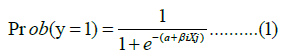
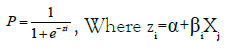
For ease of exposition, we write equation (1) as:
If Pi, the probability of a household being multidimensionally poor, is given by equation (1), then (1- Pi), the probability of a household is not poor, is
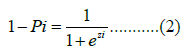
Therefore, we can write
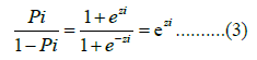
The above equation is called the odds ratio. The odds ratio gives the change in the odds of being multidimensionally poor as opposed to not being multidimensionally poor in response to one unit increase in the independent variables. Now if we take the natural log of equation (3), we get a very interesting result, namely,
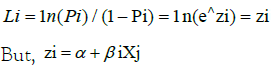
This is called a logit model where; we use it for this study as shown below.
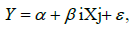
Where, i=1, 2, 3….n and j=1, 2, 3…n
Y=probability of a household being multidimensionally poor
α=intercept/constant term
βi=coefficients of the predictors
Xj= predictors/explanatory variables (Household head age, Household head sex, Household family size, Household house ownership, Household head marital status, Household employment type, Household head education, Remittance, Access to off-farm income (Households with off-farm income).
ε= stochastic disturbance term or error term
In practice, Y is unobserved, and ε is symmetrically distributed with a zero mean and has a Cumulative Distribution Function (CDF) defined as F (ε). What we observe is a dummy variable y, a realisation of a binomial process defined by
Y=1 if a household is multi dimensionally poor.
=0 otherwise
Results and Discussion
The extent of multidimensional poverty
In this section, we tried to analyse the different measures of poverty using the logistic classes of poverty indices. In order to distinguish the poor from the non-poor, a poverty line has been established based on the Multidimensional Poverty Index (MPI) method. The results of the summary of the household incidence or Multidimensional Headcount ratio (H), Intensity of poverty (A), and MPI are presented in Table 2. The MPI indices, namely head count ratio and Intensity (A) of poverty, are used to show how much the magnitude of poverty looks like in the Amhara region. Therefore, from this study, the researcher found that in urban areas, 47.3% of people are MPI poor, while in rural areas, 81.5% of households are found to be multidimensionally deprived. Thus, according to the MPI, this means that in rural areas, there is acute poverty. With regard to intensity, on average, 43% of the poor in urban areas are deprived, while rural areas account for 48.04% of the weighted indicators. Hence, society is deprived of 20.36% and 39.15%, respectively, of the total potential deprivations it could experience overall (Figure 2).
| Poverty | Urban score | Rural score |
|---|---|---|
| Multidimensional headcount ratio (H) | 0.47 | 0.81 |
| Intensity of poverty (A) | 0.43 | 0.48 |
| MPI | 0.2 | 0.39 |
Note: Source: Authors’ own computation (2023)
Table 2: Summary of Household incidence (H) and Intensity of poverty (A).

Figure 2: Magnitude of multidimensional poverty in Amhara region and among rural-urban. Note:  -Rural score.
Model’s robustness (predictive) power
The suitability of the chosen model for econometric analysis very much depends on how much it predicts from the actual observation or what % of the actual observation is really predicted by the model. There are no fixed points on which to judge the model as a good or bad predictor, yet it is generally agreed that a model with an overall predictive power of 50% or more is good. In order to assess the predictive power of the model, a classification table of correct and incorrect predictions was constructed, based on the predicted probability of being poor. The general rule of thumb in this situation is that a probability equal to or greater than 0.5 was understood as a prediction of an extremely poor household, and a probability lower than 0.5 was interpreted as a prediction of average or less extreme poverty in a household. In the table below, D stands for the number of poor households in the sample, while~D shows the number of not-poor households in the sample. The positive sign + represents the number of households predicted as poor by the model, while the negative sign-represents the number of households not predicted as poor by the model.
For instance, in rural a, the result in Figure 2, shows that 392 out of 432 poor households were correctly predicted as poor by the model. In a similar fashion, 167 out of 181 non-poor households were correctly predicted as non-poor (Figure 2). On the other hand, the off-diagonal entries of the table show that 14 non-poor households and 40 poor households were incorrectly predicted as poor and non-poor, respectively. In addition, the positive predictive value of the model, i.e., Pr(D| +), is 96.55%, which means that 96.55% of the total number of predicted poor households were in fact poor, while the negative predictive rate, i.e., Pr(D| -), is 80.68%, which implies that 80.68% of the total number of households that were not predicted to be poor by the model were in fact not poor.
In a nutshell, 91.19% of the 613 valid cases were correctly predicted by the model, and thus, the model fits the data. Similarly, the urban Model’s Predictive power for the urban poor is also shown in Annex 5.
Discussions of the result from the model
The results of the logit model are given in Tables 3-5 below, consisting of the variables, the estimated coefficients, the odds ratio, and the marginal effects for explanatory variables included in the model. The odds are the ratio of the probability of being poor to the probability of not being poor. The odds ratio gives the change in the odds of being poor as opposed to not being poor in response to one unit increase in the independent variables. The marginal effect is the percentage change in probability associated with a unit change in the explanatory variable (Table 3).
| Variables | Coefficients | Std. Err. | Z-value | Odds-Ratio |
|---|---|---|---|---|
| HH size | 0.31366 | 0.03582 | 8.76 | 1.36842 |
| Secondary edu | -1.16059 | 0.14345 | -8.09 | 0.3133 |
| primary edu | 1.50547 | 0.08624 | 17.46 | 4.50627 |
| HH Head Age | 0.01664 | 0.00248 | 6.72 | 1.01678 |
| Remittance | -0.89898 | 0.08626 | -10.42 | 0.40698 |
| Total dependency | 0.692208 | 0.06023 | 11.49 | 1.99812 |
| Unemployed | 0.639886 | 0.07661 | 8.35 | 1.89626 |
| Food price rise | 0.744544*** | 0.28988 | 2.57 | 2.10548 |
| Sex of HH | 1.219086 | 0.07906 | 15.42 | 3.38409 |
| House owned | -0.09642** | 0.08719 | -1.11 | 0.908 |
| Constants | -4.57831 | 0.19281 | -23.74 | 0.01027 |
| LR chi2(10) | 1954.72 | |||
| Pseudo R2 | 0.2774 | |||
| Prob>chi2 | 0 | |||
| Log likelihood | 2546.5503 | |||
| Sensitivity | 63.18% | |||
| Specificity | 81.63% | |||
| Correctly classified | 74.57% |
Note: Source: Authors’ own computation (2023)
**, ***Indicates the coefficients are significant at 5%, and 1% level respectively.
Table 3: Logistic results for determinants of household’s poverty: urban sample.
| Variables | Coefficients | Std. Err. | Z value | Odds-Ratio |
|---|---|---|---|---|
| HH size | 0.803391*** | 0.287358 | 2.8 | 2.233101 |
| sex of HH | 1.105015** | 0.511231 | 2.16 | 3.01927 |
| primary education | 2.574913 | 2.826675 | 0.91 | 13.13018 |
| Marital status | -0.08729 | 0.69991 | -0.12 | 0.916416 |
| Livestock Total | -1.6652 | 0.376501 | -4.42 | 0.189152 |
| HH Head Age | -0.00878 | 0.013878 | -0.63 | 0.991258 |
| Total dependency | 2.17666*** | 0.635426 | 3.43 | 8.816807 |
| Remittance | -3.41245 | 0.686867 | -4.97 | 0.03296 |
| Constants | -3.4852 | 2.378611 | -1.47 | 0.030648 |
| No_ of observations | 614 | |||
| Wald chi2(8) | 67.1 | |||
| Pseudo R2 | 0.5736 | |||
| Prob>chi2 | 0 | |||
| Log likelihood | -158.76465 | |||
| Sensitivity | 90.74% | |||
| Specificity | 92.27% | |||
| Correctly classified | 91.19% |
Note: Source: Authors’ own computation (2023)
**, *** indicates the coefficients are significant at 5%, and 1% level respectively.
Table 4: Logistic results (1) for determinants of HH’s poverty: Rural sample (1)
| Variables | Coefficients | Std. Err. | Z value | Odds Ratio |
|---|---|---|---|---|
| HH size | 0.181572 | 0.473402 | 0.38 | 1.199101 |
| sex of HH | -0.18227 | 0.958723 | -0.19 | 0.8333738 |
| Primary education | 1.512219 | 2.32795 | 0.65 | 4.536786 |
| Marital status | 2.743425 | 2.661027 | 1.03 | 15.54011 |
| Livestock Total | -1.14531** | 0.516307 | -2.22 | 0.3181253 |
| HH Head Age | -0.03631** | 0.025576 | -1.42 | 0.964338 |
| Total dependency | 2.165579** | 0.892603 | 2.43 | 8.719649 |
| Remittance | -3.00988 | 0.684196 | -4.4 | 0.0492976 |
| Marital status -widowed | 3.572908 | 2.427465 | 1.47 | 35.62003 |
| Constants | -4.69599 | 3.951936 | -1.19 | 0.0091318 |
| No_ of observations | 613 | |||
| Wald chi2(10) | 121.66 | |||
| Pseudo R2 | 0.6011 | |||
| Prob>chi2 | 0 | |||
| Log likelihood | -148.38618 | |||
| Sensitivity | 90.74% | |||
| Specificity | 92.27% | |||
| Correctly classified | 91.19% |
Note: Source: Authors’ own computation (2023)
**, *** indicates the coefficients are significant at 5%, and 1% level respectively.
Table 5: Logistic results (2) for determinants of HH’s poverty: Rural sample (2)
In urban areas, in the model, household education level, remittances, and house ownership were found to be negatively correlated with being poor. The positive coefficient of household size shows that there is a positive relationship between household size and poverty, which implies that as household size increases, the chance of falling into poverty increases. This is in conformity with the theoretical findings that large households tend to be associated with poverty. Unemployed households are more likely to be multidimensionally poor in urban areas. The variable has a positive relationship with poverty in the study area. The positive relationship indicates that households that have access to employment are less likely to be deprived than those that do not. Access to employment opportunities helps diversify and increase the amount of income received by households. In this sector, households are assumed to earn more income than those who are working elsewhere. The fluctuation in access to employment determines the poverty of urban households. The negative value of remittances shows that those households that receive remittances tend to be non-poor. The negative value household Secondary education, though not significant, implies that increasing the education of the poor will tend to reduce poverty. This is because education increases the stock of human capital, which in turn increases labour productivity and wages due to the fact that labour is the most important asset of the poor.
Age of household head: As depicted on the above Logit estimation result table, it is evident that, age of the household head is positively correlated with poverty level. Accordingly, the elderly, like pensioners, are more vulnerable to poverty in the near future. This is due to the fact that as age increases, the head faces a decline in labour supply and hence money-making or income generating capability (diminishing return).
There is a significant association between dependency ratio and poverty in a household in an urban area in the Amhara region. The more dependent members in the household, the more vulnerable the household will be to poverty, and viceversa. This means that a high dependency ratio in the household is followed by a high multidimensional poverty incidence. House ownership: there is plain evidence from Table 3, that ownership of a house is negatively associated with the multidimensional poverty of a household.
The result provides empirical support for the existing literature, for example, [32]. It is also found that a positive relationship between the sex of the household head and the probability of a household being poor implies that as households are headed by women, the probability of being poor increases. There are also large empirical findings that support the above result. For example, Chaudhuri et al. found in a study in Indonesia that households headed by women are as likely to be poor [33].
Food price rise shocks: The study shows that there is a positive relationship between food price rise shocks and poverty, which implies that as food price rise shocks increase, the chance of falling into poverty increases. The study made an effort to see the relative importance of shocks on the multidimensional poverty incidence level of a household. According to Holzmann and Jorgensen, a significant portion of households enter poverty as a result of transient shocks (such as death or higher prices) that are reversed just one or two years later [34].
Another way to analyse the effects of the independent variable on the probability of being poor is by looking at the change in the odds ratio as the independent variables change. The Table 4 below shows the odd ratios for the variables with their corresponding standard errors and confidence intervals. As shown in the table 3 above, the variables HH size, primary education, HH Head age, total dependency, unemployed, food price rise, and sex of HH have an odds ratio greater than one, which means that these variables are positively correlated with the probability of being poor. On the other hand, the variables secondary education, remittance, and house ownership all have odds ratios less than one, which means that these variables are inversely correlated with the probability of being poor.
The interpretations for odds and odds ratio: For instance, if a household head has a remittance, the odd ratio of being poor decreases by a factor of 0.407, or we can also interpret it like this: when the variable remittance increases by one%, ceteris paribus (while the values of all other variables remain unchanged), the ratio between the probability of being poor and the probability of being non-poor will be decreased by 0.407%, which implies remittances would have an impact on reducing poverty. As the age of the household increases by one year ceteris paribus (other things equal), the odds ratio of falling into poverty increases by a factor of 1.017. On the other hand, as the number of family members in the household increased by a unit, the odds ratio, keeping all other independent variables constant, increased by a factor of 1.368, which pinpoints the positive relationship between household size and poverty. As households are headed by women, the odds ratio of being poor increases by a factor of 3.384.
The educational attainment of the heads of household (in this case, secondary edu level) was found to be associated with poverty. The results obtained from the model revealed that as the heads of the household get Secondary education, ceteris paribus, the odds ratio of the household being poor decreases by a factor of 0.313, or we can say that, as the secondary level education of the household head increases by one%, ceteris paribus, the ratio between the probability of being poor and the probability of being non poor will be decreased by 0.313%. This implies that a lack of education is a factor that accounts for a higher probability of being poor. Thus, as a policy option, promotion of education is central to addressing problems of poverty, especially Secondary-level education, which was found to have paramount importance in reducing poverty in the study area (Table 4).
In rural area (Model 1 and 2), shown in Tables 4 and 5, the explanatory variables used in the model include socio economic characteristics of a household head like: sex, age, family size, dependency ratio, educational attainment (primary), remittance, marital status (widowed and married) and total livestock. The first model shows the interaction. In the model, household marital status, livestock and remittance were found to be negatively correlated to being poor.
The variables household HH size, sex of household and total dependency ratio was significantly affecting households falling in to poverty while other variables are not significant and rather inconclusive. The descriptive statistics clearly indicated that female headed households were poorer and more vulnerable to poverty. Hence the study suggests implications for gender policies. Household size was found to be positively and significantly correlated with poverty. Households with a larger size will tend to be multidimensional poor as compared to those with small size. Thus, as a remedial to this issue, family planning must be exercised among households, particularly by the poor. In this case the Amhara regional health services sector should play a critical role (Table 5).
Marginal effects after logistic regression
Since the logistic model is not linear, the marginal effects of each independent variable on the dependent variable are not constant but are dependent on the values of the independent variables [35]. As a result, in contrast to the situation in linear regression, it is not possible to interpret the estimated parameters as the impact of the independent variables on poverty. Therefore, the study estimated the marginal effect of each variable at the mean values of the independent variables. Hence, HH size, sex of HH, family size, livestock owned, and primary educational status of the household head are both significant in determining the probability of a household being poor. Table 6, below shows the marginal effects of each variable.
| Variables | Coefficients | Std. Err. | Z-value | Marginal effect (dy/dx) |
|---|---|---|---|---|
| HH size | 3.56* | 0.029 | 1.7 | 0.05 |
| Sex of HH | 1.45* | 0.037 | 1.89 | 0.067 |
| primary education | 0.013** | 0.0325 | 1.98 | 0.064 |
| Marital status | 1.94 | 0.0451 | -0.12 | -0.005 |
| Livestock Total | 0.25** | 0.045 | -2.36 | -0.105 |
| HH Head Age | 59.26 | 0.00087 | -0.64 | -0.0005 |
| Total dependency | 2.35 | 0.0341 | 4.04 | 0.138 |
| Remittance | 0.386 | 0.137 | -2.58 | -0.353 |
| Constants | -3.48 | 2.378 | -1.47 | 0.03 |
| No_ of observations | 614 | |||
| Wald chi2(8) | 67.1 | |||
| Pseudo R2 | 0.5736 | |||
| Prob>chi2 | 0 | |||
| Log likelihood | -158.76465 | |||
| Sensitivity | 90.74% | |||
| Specificity | 92.27% | |||
| Correctly classified | 91.19% |
Note: Source: Authors’ own computation (2023)
*, ** indicates the coefficients are significant at 10%, and 5% level respectively.
Table 6: Marginal Effects after Logistic Regression
The interpretation of the marginal effects: It is estimated that an additional unit in household size increases the probability of a household being poor by about 0.050, holding all other variables constant at their mean values. Having a larger household size increases the chance of falling into poverty. This finding was consistent with the research results of Sudhakara and Nega [36]. The sex of HH is significant at a less than 10% level of significance and is positively related to the probability of being poor. This shows that having a female household head increases the probability of a household being poor by about 0.067, holding all other variables constant at their mean values. One of the determinants of rural household poverty is the total livestock held by the household. As hypothesized, the livestock owned by the household has a significant and positive correlation with the poverty level of the household. An additional unit in the household level of education increases the probability of a household not being poor by 0.064, holding all other variables constant at their mean values. This implies that the risk of an individual being poor diminishes as the level of education rises.
Conclusion
Understanding the determinants and level of multidimensional household poverty would help policymakers design effective poverty alleviation policies and programs for the multi-deprived poor households and thereby difficulty to improving their living standards. The study concludes that the multidimensional headcount ratio (H), intensity (or breadth) of poverty (A), and total Multidimensional Poverty Index (MPI) were found to be higher for rural households. Further, rural households were likely to be more deprived than urban households. It also suggests that multidimensional poverty is highly concentrated among households in the lowest quintiles in Amhara regional state. In addition, household education level, remittances, and house ownership were found to be negatively correlated with being poor in urban areas. Therefore, increasing access to house-owned and educational services and qualities is important in reducing multidimensional poverty in urban areas. Similarly, sex, age, family size, dependency ratio, educational attainment (primary), remittance, marital status (widowed and married), and total livestock are also important factors that have important policy implications in rural areas for reducing poverty and meeting the MDGs.
Ethical Approval and Informed Consent Statements
“This article does not contain any studies with human participants performed by any of the authors”.
Statement of Competing Interests
The author(s) affirmed that they had no known financial conflicts of interest or personal ties that might have seemed to have influenced the work disclosed in this study.
Authors' Contributions
A, C, and D have significantly contributed the conception and design, data gathering, analysis, and interpretation of the results. The authors A, B, and C contributed to the writing of the paper or critically revised it for noteworthy intellectual content. The version that will be published has received final approval from A, B, and C. A, B, and D concur to take responsibility for all parts of the job in order to guarantee that any concerns about the correctness or integrity of any portion of the work are duly investigated and addressed. The final manuscript was read and approved by all writers.
Funding
For the research, writing, and/or publication of this work, the author did not get any financial support.
Data Availability
The data that support the findings of this study are available on request from the corresponding author.
References
- Sugden R. Commodities and capabilities. 1986:96(383) ;820-822.
- Brandolini A, Micklewright J. Measuring global poverty. Research Handbook on Measuring Poverty and Deprivation. 2023:2;60-69.
- World Bank. Classification of fragile and conflict-affected situations. Brief. 2020.
- Brian K. OECD insights income inequality the gap between rich and poor: The gap between rich and poor. oecd Publishing. 2015.
- Human Development Report HDR. 2007.
- World Bank. World Bank Group strategy for fragility, conflict, and violence 2020–2025. 2020.
- Awopeju SO. Determinants of Poverty Depth among Households in Rural Urban Nigeria. In 14th EADI General Conference: Responsible Development in a Polycentric World Inequality, Citizenship and the Middle Classes. 2014.
- Klasen S. Human development indices and indicators: A critical evaluation. Human Development Report Office Background Paper. 2018;1.
- World Bank. World Bank Group Strategy for Fragility, Conflict, and Violence 2020-2025. 2020.
- NPC (National Planning Commission). Ethiopia’s progress towards eradicating poverty: An interim report on 2015/16 poverty analysis study. 2017.
- Khandker S, Haughton J. Introduction to poverty analysis. World Bank Institute. 2005.
- Brandolini A, Micklewright J. Measuring global poverty: In research handbook on measuring poverty and deprivation. 2023:60-69.
- Chan JKN, Tong CHY, Wong CSM, Chen EYH, Chang WC. Life expectancy and years of potential life lost in bipolar disorder: Systematic review and meta-analysis. Br J Psychiatry. 2022;221(3):567-576.
[Crossref] [Google Scholar] [PubMed]
- Yimer BM, Demissie MM, Herut AH, Bareke ML, Agezew BH, Dedho NH, et al. Higher education enrollment, graduation, and employment trends in Ethiopia: An empirical analysis. 2022.
- Supply WA, Sector SA. The Federal Democratic Republic of Ethiopia Ministry of Water Irrigation and Energy. 2019.
- Agegnehu A. The cause of rural household food insecurity and coping strategy. In the case of EBINAT district, South Gondar Zone; Amhara Regional State, Ethiopia. 2015.
- Welderufael M. Analysis of households vulnerability and food insecurity in Amhara Regional State of Ethiopia: Using value at risk analysis. Ethiopian J Econ. 2015;23(683-2017-948):37-78.
- Alkire S. Multidimensional poverty measures as relevant policy tools. OPHI. 2018.
- Achenafi Y. Determinants of Urban Poverty: The Case of Gondar City, Ethiopia. 2016.
- Esubalew A. Determinants of urban poverty in Debre Markos, Ethiopia: A household level analysis. Addis Ababa University. 2006.
- Tesfaye G. Rural household’s poverty and vulnerability in Amhara region: A case study in Gubalafto Woreda. 2013.
- Merid A, Bekele D. Determinants of poverty in rural Ethiopia: Evidence from Tenta woreda, Amhara Region. Sustainable Rural Development. 2019;3(1):3-14.
- Woldie DT. Determinants of rural poverty in Banja district of Awi zone, Amhara National Regional State, Ethiopia. 2019.
- Neway MM, Massresha SE. The determinants of household poverty: The case of berehet woreda, Amhara regional state, Ethiopia. Cogent Econ Finance. 2020;10(1):2156090.
- Eshetu S, Gian S. Determinants of farm household poverty status in South Wollo zone, Amhara regional state, Ethiopia. Eshetu Seid 1. Int J Res Econ Soc Sci. 2016;6(11):322-329.
- Kassaw T. Magnitude and determinants of rural household poverty in Ebinat district of Amhara National regional state of Ethiopia. 2020.
- Endalew B, Tassie K. Determinants of rural household poverty across agro-ecology in Amhara region, Ethiopia: Evidence from Yilmana Densa Woreda. J Econ Sustain Dev. 2018;9(7):87-97.
- Mulugeta S. Determinants of urban poverty: A household level analysis in case of DEBRE Birhan Town, Ethiopia. (Doctoral dissertation). 2019.
- Ermiyas A, Batu M, Teka E. Determinants of rural poverty in Ethiopia: A household level analysis in the case of Dejen woreda. Arts Social Sci J. 2019;10(2).
- World Bank. Ethiopia Socioeconomic Survey 2013-2014. Living Standards Measurement Study. 2015.
- Alkire S, Santos ME. Multidimensional Poverty Index (MPI). Oxford Poverty and Human Development Initiative (OPHI). 2010.
- Apili M. An investigation on the impact of poverty on female-headed households in Kangai Sub County, Dokolo district of Northern Uganda. 2019.
- Chaudhuri S, Jalan J, Suryahadi A. Assessing household vulnerability to poverty from cross-sectional data: A methodology and estimates from Indonesia. 2002.
- Holzmann R, Jorgensen S. Conceptual underpinnings for the social protection sector strategy paper. Putting People at the Center of Sustainable Development. 1990;45.
- Rodriguez A, Furquim F, DesJardins SL. Categorical and limited dependent variable modeling in higher education. Higher Education: Handbook of Theory and Research. 2018;295-370.
- Babu S, Reda NA. Determinants of poverty in rural tigray: Ethiopia evidence from rural households of Gulomekeda Wereda. Int J Sci Res. 2015;4(3):822-828.
Citation: Mulusew A, Hong M, W/rufael M, Kesete M, (2023) Determinants of Household Poverty: Analysis of Multidimensional Aspect in Rural and Urban Areas in Amhara Regional State, Ethiopia. Review Pub Administration Manag. 11:431.
Copyright: © 2023 Mulusew A, et al. This is an open-access article distributed under the terms of the Creative Commons Attribution License, which permits unrestricted use, distribution, and reproduction in any medium, provided the original author and source are credited.