International Journal of Swarm Intelligence and Evolutionary Computation

Deep Learning Algorithm (2024)

N Nafati^*, F Paris and E Huyghe Department of Computer Science, Toulouse University Hospital, Toulouse, France
^*Correspondence: N Nafati, Department of Computer Science, Toulouse University Hospital, Toulouse, France, Email:

Received: 26-Dec-2024, Manuscript No. SIEC-26-28000; Editor assigned: 30-Dec-2024, Pre QC No. SIEC-26-28000 (PQ); Reviewed: 13-Jan-2025, QC No. SIEC-26-28000; Revised: 10-Sep-2025, Manuscript No. SIEC-26-28000 (R); Published: 17-Sep-2025, DOI: 10.35248/2090-4908.25.14.431

Introduction

Deep learning is an essential subfield of AI (Artificial Intelligence). This concept is based on machine learning through complex neural networks. This advanced field of machine learning offers a deep understanding of algorithms inspired by the neural network of the human brain. It excels at solving complex tasks, ranging from computer vision, natural language …, to biological data understanding [1,2].

Description

Difference with machine learning (Automatic learning)

A neuron can be schematized as shown in the Figure 1 [3].

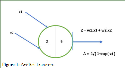
Figure 1: Artificial neuron.

Z=W × X+b in matrix form and it is the forward propagation

A being the activation function

x₁, and x₂ are two vectors columns of input of dimension m

Where b is the column vector noise

W₁, where W₂ is the weighting weights of x₁ and x₂, respectively, to be optimized

The log loss function to minimize

The cost function to be minimized is given by the following formula:

Where Y is the binary variable known as a vector of dimension m.

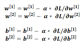
Then comes the optimization to minimize the cost function by going through the descent of the gradient. Gradient decent, and updated W and b (noise) parameters it is the back propagation such as:

In the backpropagation comes the optimization to minimize the cost function by going through the descent of the gradient. Gradient decent, and updated W and b (noise) parameters such as:

The update is done by going through the gradient such as:

In a neural network, the path of input features transformed into output after passing through one or more hidden layers, and the output layer is called forward propagation process.

Algorithm of deep learning

Parametres=Matrix Parameter Initializations (Inputs)

For layer in range (n_iter) do

Activations=forward-propagation ()

In a neural network, the path of input features transformed into output after passing through one or more and through hidden layers, and the output layer is called forward propagation

Gradients = back propagation ()

Backpropagation consists of going in the opposite direction to adjust the weights of the nodes in order to decrease the error. The same process is repeated until the desired output is obtained.

Parameters=update (gradients, parameters, learning rate) end.

Learning curve

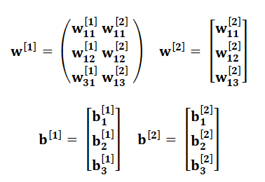
Example of two-layer neural networks

Diagram of two-layer neural network shows in Figure 2.

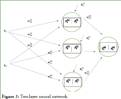
Figure 2: Two-layer neural network.

The learning curve (Figure 3) is downward at the beginning and flat towards the end, with the cost per unit represented on the Y axis and the total output on the X axis. As learning increases, the cost per unit of output initially decreases before flattening as it becomes more difficult to increase the efficiency gained through learning out as it becomes more difficult to increase the efficiency gained through learning.

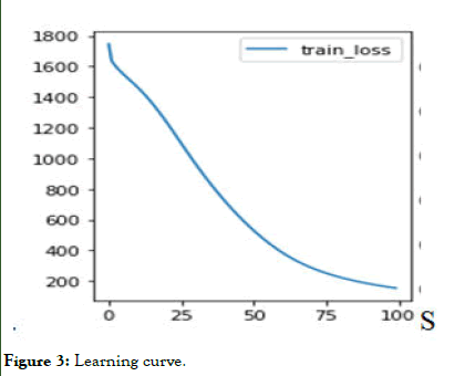
Figure 3: Learning curve.

Validation curve: Exactitude

Exactitude measured by the deviation of the results from the "true" value. Combination of fidelity and exactitude y. Total error; It is not because we have a faithful and fair method that it is automatically exact. It is therefore necessary to check the exactitude in the end (Figure 4) [4,5].

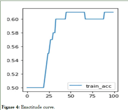
Figure 4: Exactitude curve.

Exactitude is a metric for evaluating the performance of classification models with 2 or more classes. Exactitude can be translated as "precision" in French.

Like other metrics, exactitude is based on the confusion matrix. As a reminder, the confusion matrix is composed of 4 values (True negative, false negative, false Positive, true positive).

Deep learning image result

Accuracy makes it possible to describe the performance of the model on positive and negative individuals in a symmetrical way. It measures the rate of correct predictions on all individuals.

Accuracy makes it possible to describe the performance of the model on positive and negative individuals in a symmetrical way. It measures the rate of correct predictions on all individuals (Figure 5).

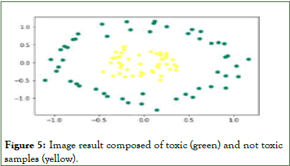
Figure 5: Image result composed of toxic (green) and not toxic samples (yellow).

Conclusion

Machine learning and deep learning are two types of Artificial Intelligence (AI). Machine learning is AI that can adapt automatically with minimal human interference, and deep learning is a subset of machine learning that uses neural networks to mimic the learning process of the human brain.

Our algorithm uses deep learning to classify input data into two groups, toxic and non-toxic.

References

1. Kapoor A, Gulli A, Pal S. Deep learning with TensorFlow and Keras: Build and deploy supervised, unsupervised, deep, and reinforcement learning models. 2020.

   [Google Scholar]

2. Collobert R. Deep learning for efficient discriminative parsing. 2011;95–102.

   [Google Scholar]

3. Tahew A, Arul A, Sivakumari S. Deep learning techniques: An overview. 2021.
4. Schmidhuber J. Deep learning in neural networks: An overview. Neural Networks. 2015;61:85–117.

   [Crossref] [Google Scholar] [PubMed]

5. Gulshan V, Peng L, Coram M, Stumpe MC. Development and validation of a deep learning algorithm for detection of diabetic retinopathy in retinal fundus photographs. JAMA. 2016;316(22):2402–2410.

   [Google Scholar]