Journal of Petroleum & Environmental Biotechnology

Rock Typing by Bulk Volume Water Method in the Carbonate Reservoirs

Zahra Riazi^* Department of Infrastructure Engineering, University of Melbourne, Melbourne, Australia
^*Correspondence: Zahra Riazi, Department of Infrastructure Engineering, University of Melbourne, Melbourne, Australia, Email:

Received: 07-Jan-2022, Manuscript No. JPEB-22-15416; Editor assigned: 12-Jan-2022, Pre QC No. JPEB-22-15416(PQ); Reviewed: 25-Jan-2022, QC No. JPEB-22-15416; Revised: 01-Feb-2022, Manuscript No. JPEB-22-15416(R); Published: 08-Feb-2022, DOI: 10.35248/2157-7463.22.13.451

Nomenclature

A͞ : Average of IWS and Porosity Product in the Specific Group; BVW: Bulk Volume Water; k : Permeability, mD; CCAL: Conventional Core Analysis; DRT: Discrete Rock Type; FZI: Flow Zone Indicator, μm; MLP: Modified Lorenz Plot; MICP: Mercury Injection Capillary Pressure, psi; P_d: Displacement pressure, psi; : Entry pressure, psi; P_t: Threshold pressure, psi; RFN: Rock Fabric Numbers, RQI: Reservoir Quality Index, μm; φ : Porosity, (fraction); S_Wri: Irreducible Water Saturation, %; SCAL: Special Core Analysis; SFP: Stratigraphic Flow Profile; SMLP: Stratigraphic Modified Lorenz Plot; SWPH: Product of IWS and Porosity.

Introduction

According to the classical definition, rock typing is reservoir rock classification into distinct units, which were each deposited under similar conditions and experienced similar diagenetic processes. This results in a unique porosity-permeability relationship and similar capillary pressure profile for each rock type [1]. This definition considers different reservoir properties either in the shape of characteristics or relationships for knowing a definite rock type. So, every acquired data (RCAL, SCAL, well log interpretation, and well test results) can be applied for this classification and can complete it regarding its scale. Acquaintance with these distinct units can be started using small scales data (thin sections and core data), their extent and sequence along the wells followed by petrophysical logs and distributed throughout the reservoir using seismic data. Dynamic rock typing is done on upscaled data (formerly classified as static rock typing) and model is initialized with the capillary pressure curves allocated to defined rock type, then the oil in place is estimated. Consequently, all predictions and results of defined dynamic scenarios are influenced by the defined rock types. This clearly reflects its importance during reservoir study and its modelling. Indeed, existing different rock typing methods that classify reservoir rock qualitatively (e.g., different Lorenz and Stratigraphic Plots and quantitatively (e.g., Winland plot, RQI and BVW) have been developed to address this need.

Permeability and porosity are the main inputs for the most rock typing methods, while source of permeability data is limited to few wells and intervals in the whole reservoir. Rock typing process is limited to these intervals, but it needs to distribute them to all wells and intervals. The applied methods relay on porosity and common log variables, which exist for all intervals. In the simple case, porosity and permeability correlation in the cored sections is applied for un-cored section using log porosity. Though, log porosity needs to be matched with porosity at the cored depths and in the case of carbonates this correlation has low correlation coefficient. Existing secondary porosity and fractures in the carbonate reservoirs decrease correlation coefficient in both core porosity-log porosity and core porosity-permeability data correlations.

Some methods like generating correlation between the combination of log data and Flow Zone Indicator (FZI), Discrete Rock Type (DRT) or artificial neural network have been used to rectify this issue. However, applying these methods, beside their complexity, imposes more uncertainty into the models [2-4]. Also, they usually present very low correlation coefficient for the known points when they act as the control points for produced results. Therefore, the predicted permeability usually suffers from enough accuracy and the problem of feeding the outcomes to the static and dynamic models still exists in these methods and seems improper to apply for carbonates.

Generally, rock typing in carbonates has been challenging due to existing great diversity in both size and shape of grain for the most carbonate sediments in comparison with sandstones. Existing post-sediment diagenetic processes and facies changes lead to pore size variations from micron to cave size and complexity of their networks. These influence porosity and permeability relationship with decreasing their correlation coefficient, which is high in the sandstones. In other words, a vuggy porosity can store significant volumes of oil, but existing poor connection between the vugs may lead to the low permeability and production.

On the other hand, the BVW method uses Irreducible Water Saturation (IWS) and porosity, which are available along well column and solve the problem of data scarcity. Moreover, existing log porosity and water saturation help to directly feed the result of rock typing to the static and dynamic models. This eliminates the need for intermediate methods that may increase model uncertainties. Theoretically, using water saturation as the input of the BVW method reflects the effect of pore throat size, which is the controlling factor in carbonate reservoirs for flowing the fluids and is common factor with permeability. Also, applying both BVW and RQI methods in a carbonate field and comparing the outcomes using grouped MICP curves disclosed more similarity between the grouped MICP curves by BVW method than RQI [5]. Despite these benefits, this method has been rarely applied for rock typing as a stand-alone method. It has been presented in the literature as an auxiliary method with other approaches during rock typing, but not considered as a standalone method for this purpose. For example, Winland’s plot versus Bulk Volume Water (BVW) was used for rock typing or irreducible water saturation in its formula was substituted with the general model between porosity, permeability and irreducible water saturation [6,7]. This study tried to consider capacity of this method as an independent one to classify reservoir rocks using three carbonate field data.

This paper examined applicability of BVW method after a short explanation about the methodology of the BVW method and its algorithm for coding. Next, the rock typing outcomes were validated by MICP curves in the “Results” section. Finally, applying this method was discussed in comparison with RQI and FZI method, which utilizes permeability and porosity as its input, in the last section.

Methodology

Bulk Volume Water (BVW) is the product of water saturation and porosity, which presents the fraction of occupied porous volume by water in the reservoir rock. Above the transition zone, this water saturation is equivalent to Irreducible Water Saturation (IWS), which is immovable during production. This fraction of water is bounded within the pore network by capillary force and adsorbed onto grain surfaces. Capillary pressure is controlled by pore throat network diameter, which is a random variable and depends on grain size. Decreasing or increasing the pore throat network radius leads to rising or reducing capillary pressure, respectively and has a contrary effect on the percentage of IWS in the reservoir rock. The BVW method classifies reservoir rock based on this concept, the fraction of water in reservoir rock reflecting different pore throat sizes. In other words, in the depths with similar rock properties are expected relatively a similar value of product of porosity and water saturation as the BVW, which classify these depths as a same rock type.

Hypothesized a similar relation between porosity and connate water saturation with considering the similarity between “surface area-diameter of the particle” and “surface area-porosity” correlations [8]. He used the inter-relationship between porosity and mean particle diameter and attained the equilateral hyperbole relationship between saturation and porosity, which expresses the IWS as a fraction of bulk volume instead of pore volume:

This is a recognized concept in the oil industry and its plot (Buckles plot) is typically applied for different reservoir parameter evaluations. This plot includes a family of hyperbolic curves, in which each one shows a constant BVW value, increasing this constant value has opposing relation with pore throat size (Figure 1). Several applications for this method and recapped them: discretising reservoir zone with IWS; estimation of water-cut and producibility; Permeability prediction; grain size approximation; pore type estimation; detection of multiple lithology [9,10]. The four last applications of the BVW methods are related to rock typing. Indeed, for a reservoir with variable lithology, this family of curves are formed by a selective classification of data, which determine rock types.

Figure 1: The bulk volume water plot.

The dependency of water saturation on pore throat size inter relates the BVW method to the capillary pressure. Capillary pressure, as the opposing force during oil migration, is controlled by the distribution of pore throat radius in the reservoir rocks, which is generally estimated by a MICP curve in a rock sample (Figure 2).

Figure 2: Different sections and points in a MICP curve [11].

Normally, an MICP curve has two main sections, a plateau and steep slopes, which shows arriving mercury in the macro pores and micro pores, respectively [11,12]. The plateau section forms in lower mercury saturations and its slope infers the quality of pore throat sorting in the rock sample. A horizontal shape reflects a good and uniform pore-throat size sorting; while, steeping the plateau infers deteriorating pore-throat structure [13]. The plateau joins to the steep section of the graph, which ends at the highest capillary pressure. Tangent line to the highest-pressure section of MICP curves is parallel with y-axis and indicates the percentage of pore space in the rock sample, which mercury could not invade and its corresponding saturation spots IWS in the sample.

Pe, Pd, and Pt are definite pressure points on the MICP curves which indicate entry, displacement, and threshold pressure, respectively. Pe is influenced by irregularities that may exist around the sample surface. These irregularities cause mercury to arrive in the space between them and sample holder and this extra saturation must be corrected before using the curve. Pd shows the amount of pressure that a non-wetting fluid requires entering the largest connected pore throats in the rock sample [14]. Finally, Pt indicates the pressure that mercury forms a connected pathway along the sample [15].

Indeed, different sections of a MICP curve provide either qualitative or quantitative information about pore throat sizes, sorting, and the IWS for a reservoir rock sample. These are main factors, which help during reservoir rock classification process. Moreover, the size and sorting of pore throats are general factors between permeability and hydrocarbon saturation and can relate these two variables. Therefore, information infers from an MICP curve makes it an appropriate source for both reservoir rock typing and verifying other quantitative rock typing approaches.

Bulk volume water rock typing method application

This methodology is applied by data selection from some candidate wells and using their log porosity and water saturation at the depth above the transition zone. In this zone initial water saturation depends on both reservoir rock properties and fluid contacts, which this limits reservoir rock classification merely based on its properties. So, before using the data, it is recommended to draw log porosity and saturation versus depth and omit the transition data visually. The Buckles Plot can help to remove points in the border of oil and transition zones. Following, to prevent discarding any data point corresponding to the net rock volume, conservative cut-off values can be applied for both porosity and water saturation.

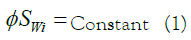
After applying data preparation stage, reservoir rock typing is commenced with multiplying porosity and water saturation values. This product is sorted from minimum to maximum and classification is begun from the minimum point. Next, a group of data is chosen from this data set, as the first rock type, and averaged ( ) and “ ” value are calculated with the following formula for each data in this group. Then, the “ ” is checked for all data in the group to be in the defined limit. In the case of being the limit, the first rock type is defined.

The value of “ ” should be in a certain range of 0.8 to 1.2 for each data point. This shows its similarity to the average property of selected group. In the other words, the property of each point needs to be near to the average of group for being supposed as a member of a rock type. If the “ ” value is less/more than this range, the selected series should be changed until meeting the mentioned condition. With finding a group, which its members have “ ” value in a range between 0.8 to 1.2 a rock type is distinguished between all data. This procedure should be repeated with selecting next group and classifying the rest of the data. Following, it was recapped this process in its algorithm:

1. Calculate product of “φS_Wir ”.

2. Sort “ ” data from Min to Max.

3. Choose a new range of sorted data and averaged over this range ( A͞ ).

4. Calculate for all data points in the chosen range:

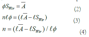
5. Check has a value between 0.8 and 1.2.

It is in the mentioned range; one rock type is formed. Repeat the procedure for next.

It is not, change of the range to include more (or less) data points to satisfy the criteria of values.

The grouping data procedure for separating different rock types is done by trial and error in the BVW method, which can be its only pitfall and can be challenging in the case of huge amount of data. So, a computer code was prepared based on the mentioned algorithm by MATLAB to solve the trial-and-error process in this method. The code was verified using three carbonate fields and applied for their reservoir rock typing, which has been discussed in following section.

Feeding the rock typing results to the static and dynamic models is very fast and convenient by this method in comparison with other usual rock typing approaches. In the case of using the software, it needs to follow succeeding steps:

1. Build two new variables; firstly, with general template showing product of IWS and porosity; the second one, with the discrete template as the saturation region identifier.

2. Using calculator option in this software, assign the multiplication of initial water saturation and porosity to the new defined property.

3. Again, by calculator and maximum and minimum of each rock type, fix different rock type in the variable that was defined with discrete template.

Case studies

The prepared MATLAB code was examined by three carbonate fields data. The Sarvak, Fahliyan, and Kangan-Dalan are carbonate formations in the fields A, field B and field C, respectively. The porosity and water saturation data resulted from log interpretation were selected from three wells for each field. For data preparation, the data points, which were in and below the transition zone, were omitted using resistivity and porosity logs and the result was checked by the Picket plot. As the final step, the cut-off values of less than 5% and more than 70% were applied for porosity and IWS data, respectively in the three fields. Based on cut-off value estimation in these fields, applying mentioned values do not influence original oil in place value.

For each field, the prepared data (porosity and water saturation) were fed to the MATLAB code and result of rock type classification was presented in Figures 3-7. The MICP curves in each field were used to investigate the accuracy of results. The MICP curves were classified based on position of their porosity and IWS in the rock types’ plot. Since Field A is a newly developed field, it lacks the SCAL data and MICP curves from its nearby field were applied for its rock typing verification.

Figure 3: Rock type classification by BVW method in Field A.

Figure 4: Classified MICP curves (A) and porosity vs permeability (B) based on defined rock types in the Field.

Figure 5: Rock type classification by BVW method and comparing its results with MICP data in field B.

Figure 6: Grouping the MICP curves (A) and its Porosity-Permeability correlation (B) based on BVW in Field B.

Figure 7: Rock type classification by BVW method and comparing its results with MICP data in field C.

Results

Case 1: Field A

Sarvak formation with the middle cretaceous age is the oil-bearing formation in the Field A and is known as the age-equivalent of the Mishrif and Natih formations. It composes of limestone to argillaceous limestone and were strongly affected by diagenesis, some tectonic, and paleo-topography events. Sarvak formation in this field is divided into nine subzones from very poor due to the occurrence of shaly layers in the Zone 1 and Zone 2 to the high porosity and medium permeability limestones in Zone-3. Quality of Zone-4, Zone-5 and Zone-6 varies throughout the field from weak to medium in comparison with Zone-3. The oil-water contact has tilted shape from north to south of field. Increasing water saturation starts from end of sarvak-7 in some place or middle of Sarvak-8 and Sarvak-9 is completely water-bearing zones.

Figure 3 displays results of rock typing by the MATLAB code, which classified porosity and water saturation to four rock types in Field A. As the figure shows rock type 3 and rock type 4 have more frequency, which referring to Figure 1 reflects medium to poor average pore sizes. The reservoir section with high quality is shown by rock type 1 and rock type 2.

Rock types were verified by MICP curves; so that, their initial water saturation and porosity were inserted in the rock type plot (green circles in the Figure 3). Then, they were grouped in the next step regarding their position in classified rock types (Figure 4A).

Clustered MICP curves in the Figure 4A display good separation especially in the high-pressure values that indicates initial water saturation. Based on different sections of a MICP curve (Figure 2), the existing MICP curves in each group present relatively similar characteristics as the member of one cluster indicated by a rock type. Moving from the first (blue colour points) to the fourth rock type in Figure 3 and comparing with the shape of MICP curves in their related rock type (shown by similar colour), reveal good consistency between them. The first group of MICP curves show vertical steep slope and their flat plateau section indicates a good and uniform pore-throat size sorting for this rock type. Also, they present the least initial water saturation in comparison with the curves in other groups. This presents coarser pore throat size that is consistent with the position of the first rock type in the Buckles plot. Decreasing average pore sizes from the second to the fourth rock types agrees with the existing variations in the MICP curves for their equivalent group.

Since the IWS and porosity display hyperbolic relationship in the Buckles plot, it is expected to see some changes in the shape of MICP curves for each individual rock type. Indeed, with moving in direction of high saturation-low porosity to low saturation- high porosity points, the MICP curves show lower initial water saturation and threshold pressure.

Porosity and permeability correlations for different rock types are displayed and indicated by “RT” in Figure 4B. Considering all in one graph presents neither specific correlation nor clear separation between them for different rock types. However, there is an overall increasing trend between porosity and permeability of each rock type, but they cover each other. In other words, porosity- permeability correlation of MICP samples in each rock type relatively corresponds with its reservoir properties in Figure 3; although, they show no clear separation between themselves. Existing different types of secondary porosity in the carbonates (vugs, fissures and fractures) influences shape of increasing trend between porosity- permeability correlation. A very dense samples with low porosity can present high permeability in the case of having fissures in its structure or in the opposite shape, non-connected vugs form high porosity but low permeability. In these situations, shape of pore throat network in a MICP curves would determine the real type of rock sample.

Case 2: Field B

Fahliyan formation with the late Cretaceous age is the main reservoir in the Field B. This carbonate formation was deposited in the Zagros sedimentary basin and it is a part of Khami Group. Its thickness is about 1312 ft and was divided into four members in this field. The members have different thicknesses and oil presents in all of them. They mainly consist of limestone, occasionally claystone or dolostone, with local argillaceous limestones, which are separated by low-permeability layers.

Applying the BVW method on log porosity and water saturation data of Field B, classified its carbonate reservoir rock into three different rock types (Figure 5). Rock type 2 allocated the most data to itself, but it is placed in the position of rock type 3 in the Field A (Figure 3). Following, the porosity and initial water saturation of MICP curves were inserted (green dots on Figure 5) on the rock types’ plot and categorized based on their position (Figure 6A). As the Figure 5 shows, more data points were used in the Field B; though, they did not cover whole hyperbolic shape of IWS-porosity correlation uniformly.

Considering MICP curves in each group presents a clear similarity between them, especially regarding their IWS. Related MICP curves to the rock type 1 display relatively a flat plateau, which infers a good sorting. The plateau section of curves inclines in the rock type 2 and is steeper for rock type 2, which reflects deteriorating pore- throat sorting in these types of reservoir rock samples. Also, the inflection point occurred at lower capillary pressure for the MICP curves in rock type 1, while it increased for the rest and leaded to the grouped MICP curves with the higher IWS in rock type 2 and 3.

Figure 6B presents porosity-permeability cross plot for the classified MICP curves in the Field B. The plot displays an increasing trend between porosity and permeability for each rock type, while they covered each other.

In comparison with the Field A, the porosity-permeability cross plot presents more scattering between porosity and permeability data of different rock types. Data points can graphically be divided into two general increasing trends (black dashed line on the Figure 6B). These infer two general slopes for the porosity and permeability correlations. In the left section of dashed line, permeability improves corresponding to the porosity increment, while in the right section the rate of permeability enhancement seems slower with increasing porosity. The second group can present unconnected vuggy porosity in the related rock samples in addition to the intergranular porosity. In the other words, the porosity enhanced more than two times, but the permeability barely raised more 8 mD.

Case 3: Field C

The Kangan and Dalan are Late Permian formations and the members of Dehram Group, which is correlated with the Khuff formation. The Kangan overlies the Dalan formation, and it consists of clean carbonate, basal argillaceous, and evaporite carbonate facies. Limestones and evaporites of the Dalan formation in the studied area, are subdivided into three primary members including the upper and lower Dalan (mainly limestone, dolomitic limestone) and Nar evaporites (anhydrite and thin interlayers of dolomite) in the middle.

According to the log data (porosity and water saturation) in three wells and the BVW method, carbonates were classified to three rock types in the Field C with the most frequency for rock type 3 (Figure 7).

Inserting the IWS and porosity of MICP samples into the rock typing plot (green circles Figure 7) present a good coverage of MICP data points for Rock type#1 and 2. Therefore, it is expected to see various shapes of MICP curves for these two classes.

Clustered MICP curves and their porosity-permeability correlations were plotted for three rock types in Figure 8A and 8B, respectively. Similar to the Field B, existing small-scale heterogeneities in the reservoir samples formed the MICP curves with variable plateau or steep sections. Thus, despite of belonging to different rock types, some MICP curves covered each other at the low-pressure section. Moving from rock type 1 to 3, the plateau section of MICP curves started at higher entry pressure and their shape could not preserve their consistency with increasing saturation. The curves related to the rock type 1 presented more uniform and flatter plateau section, which inclined to one or more slopes in the rock type 2 and 3. This deduces decreasing both pore-throat size and uniformity in macropores and increasing percentage of micropores in the samples from rock type 1 to 3. This was confirmed by their porosity-permeability correlations (Figure 8B). For instance, despite of enhancing porosity from 0.05 to more than 0.3 in the MICP samples of Rock type #3 (yellow dots), permeability changed from 0.3 mD to 7 mD. These can present existing non-connected vugs, which more affected porosity.

Figure 8: Grouping the MICP curves using BVW method (A) and Porosity- Permeability correlation (B) for the Field C.

Overall, plotting porosity-permeability correlations of MICP data for defined rock types in Field C displayed no separation between themselves and cover each other (like Field A and B). Though, the MICP points can be categorized hypothetically into three general groups (dashed lines in Figure 8B) regarding porosity-permeability relationship. They show an increasing trend in these groups but with different slopes and all three rock types were distributed in them. Indeed, the points in the left, middle, and right sections can deduce existing fracture, intergranular porosity, and non-connected vugs in their related rock sample, respectively. Therefore, in this situation, using pore throat network can be more appropriate parameter for rock type classification. Since it can reflect type of rock using its shape and initial water saturation, which are the outcome all existing variations in the rock sample that may affect porosity value.

Discussion

Comparing the BVW method for carbonates with other methods using permeability as their input, was utilized the RQI method. This method was broadly explained in the literatures and was not mentioned here to avoid repetition [2,5].

Applying the RQI method, the porosity and permeability of MICP samples were used as the inputs for these three fields. This makes easier comparison between the outcomes of two methods. The porosity and permeability data were clustered using the RQI method in the three fields. Then, the related MICP curves were gathered in different groups based on similar FZI value. Figures 9-11 presents outcomes of these two steps for Field A, B, and C, respectively in two subplots of C and D.

Figure 9: Classifying Porosity- Permeability and MICP curves using RQI/FZI method (Field A).

Figure 10: Classifying Porosity- Permeability and MICP curves using RQI/FZI method (Field B).

Figure 11: Classifying Porosity- Permeability and MICP curves using RQI/FZI method (Field C).

Looking at the outcomes of rock typing by the BVW (Figures 3, 5, and 7) and RQI (Figures 9, 10, and 11C) methods reveal both classified carbonates to four rock types in Field A. For Field B and C, the RQI method classified carbonates into six rock types; so, it is expected to see more similarity between the MICP curves related to each rock type in comparison with three rock types using the BVW method.

Overall, clustered MICP curves based on four rock types defined by RQI method (shown by same colour of related rock type) display no clear separation in Figures 9C and 9D in the Field A. The MICP curves belong to each rock type were spread along the plot and covered the other rock types’ curves (Figure 9D). This pattern was repeated for the Field B and Field C (Figures 10 and 11). Indeed, the porosity and permeability data display distinctive correlation for each rock type using RQI method, but their related MICP curves cover each other without any clear separations. Comparing them with the outcomes of the BVW method (Figures 4, 6, and 8A) presents more mixing pattern despite more rock types, while separation between the clustered curves by the BVW method is clear.

Investigating the outcomes of classifications with more precision, the classified curves were detached in subplots (Figures 12-14). Field A with equal number of rock types by two methods presents more similarity between the clustered MICP curves by the BVW. Although, these resemblances were faded in the rock types were grouped by the RQI method (Figure 12). For the Field B and C (Figures 13 and 14) similarity between the curves by the BVW in the Field A was converted to some sort of variations. Although, except the last rock types, inequality in plateau, and steep slopes of the MICP curves are not notable in each rock types and all were slain in the limited range of IWS value. In comparison, the grouped MICP curves by the RQI in the Field B and C (Figures 13 and 14) indicated extensive variations for each rock type. Nevertheless, some sort of similarity presents only for rock type 1 and 5 in Field B (Figure 13), the rest display inequality in different sections of MICP curves, which leaded to scattered IWS in them.

Figure 12: Classified MICP curves using the BVW and RQI/FZI methods (Field A).

Figure 13: Classified MICP curves using the BVW and RQI/FZI methods (Field B).

Figure 14: Classified MICP curves using the BVW and RQI/FZI method (Field C).

Possible source of these dissimilarities between the MICP curves in a defined rock type can be discussed regarding two aspects. One can be related to their mathematical relationship, which exists between their variables. This puts two curves in one group, while presenting relatively same shape but different values in the specific points (e.g., IWS). The other connects distortions in the regular shape of an MICP curve to the existing heterogeneities and secondary porosity in the carbonate rock samples.

Technically, both the RQI and BVW methods classify reservoir rocks using a relationship between two reservoir parameters. These are quotient of permeability-porosity and multiplication of IWS and porosity, respectively. Indeed, in these two methods, their related variables can vary in their ranges, while the results of calculations can be the same. In other word, division of high permeability and porosity that is used in the RQI method can result same value as both are low. The same situation, but in shape of multiplication exists for the BVW method. Multiplying low porosity and high IWS can be equal to high porosity and low water saturation. This leads to existing different shapes of MICP curves for one rock type, which reflect presence of two opposite limits in each rock type. However, it seems application of cut off on the log porosity/IWS and the shape of grouping in the BVW method (Figure 1), which distribution of rock types gets narrow at the two ends for each group, alleviate this problem in it.

Existence of more than one pore throat distribution group in a MICP sample can be a common feature in the carbonates due to secondary porosities, and small-scale heterogeneities (e.g., micro scale facies change). Each distribution group presents specific value regarding the saturation, during invasion of mercury at a definite pressure. These distort the regular shape of MICP curves and formation of different inflection points in the plateau and steep sections of a MICP curve can clearly present them.

Therefore, depending on the rang of variables for each rock type and presenting secondary porosity or heterogeneities in a carbonate reservoir rock, possibility of seeing different shapes for the MICP curves changes in a rock type. Although, existing a wide range for variables interrelates to the function of secondary porosity in the carbonates. In this situation, similarity between different sections of the MICP curves can be applied as the grouping criteria and optimizing number of groups (e.g., similarity between IWS, slope of plateau section).

As the Figures 3, 5, and 7 display the range of porosity and IWS changed for different rock types classified by the BVW method. Their ranges increase especially for the water saturation with decreasing pore throat size. Therefore, it is expected to see more variation in the shape of MICP curves that exist in the last two rock types. Looking at MICP curves related to these groups (by the BVW) in Figures 12-14 clearly present these variations; though, some sort of similarity is distinguishable between them.

In the case of the RQI method, range of permeability extended more than ten times for a rock type. Moreover, due to existing secondary porosity in the carbonates (non-connected vugs or microfracture), increasing either porosity or permeability may not be correlated with each other. These caused more variations in the shape of MICP curves for a defined rock type by this method. For the Field A, porosity and permeability of rock types vary from 0.4 mD to 100 mD and 0.05 to 0.3, respectively (Figure 9C). So, as it is expected, the MICP curves with different shapes and curvatures exist for each rock type (Figure 12). Although, the rock type 1 with a limited range of variables showed some sort of similarity between its curves, others contain curves with variable shapes and IWS values. Considering the porosity-permeability correlations in Figures 10C and 11C reveals, they expanded in the wide ranges for each rock type. Therefore, the clustered MICP curves based on these rock types presented variable shapes and values; despite higher number of rock types by the RQI method (Figures 12 and 13).

The grouped MICP curves using the BVW and RQI methods can be compared by considering dissimilarity and likeness both in the plateau, and steep slopes of curves presenting the macropores and micropores condition, respectively and ultimately IWS in the sample. Starting with plateau and slope sections of MICP curves, homogeneity between these two sections for the ones grouped by BVW in comparison with RQI method is completely clear for Field A (Figure 12); although, outcomes of the BVW method showed better performance. Overall, some curves show a stepwise shape either in the plateau or slope sections due to inhomogeneities in the MICP samples for the Field B and C. Forementioned, sloping the plateau section from a horizontal shape infers deteriorating pore-throat structure from a uniform shape, and this works for all sections. Therefore, these curves can only be compared by IWS as the grouping criteria, which is their final condition at high capillary pressure.

Using IWS as the grouping criteria and pondering outcomes of two methods by this reveals more homogeneous grouping results for the BVW method. Although, there are few rock types classified by RQI method that show a limited range for IWS (RT 1 and 5 for Field B), but in comparison with the outcomes of the BVW presented clustering with more disparate members. Moreover, the number of rock types is less in using the BVW method. Effect of number of rock types gets prominent when they are applied for property distributions in the static model and dynamic modelling.

Generally, rock typing process is finalized by reporting rock type limits, a capillary pressure, and two relative permeabilities curves (water-oil and gas-oil) as the representative of all existing curves for each rock type. In this step, lack of optimum number for the rock types usually results very similar representative capillary pressure curves for the middle rock types. This problem is added to the existing challenge during feeding the rock types to the models. Moreover, generating representative relative permeability curves for all rock types is challenging and sometimes seems unreal for some rock types. So, it is essential to keep balance between the number of rock types and similarity between the members for each rock type.

Conclusion

Existing secondary porosity either in the shapes of unconnected vugs or microfracture and facies changes in different scales form a wide range of variations in the reservoir rock properties leading to the weak correlation between porosity and permeability data for the carbonates. Therefore, the classification outcomes using any method applies relationships between these two reservoir parameters cannot satisfy expecting result for the rock type clustering.

Applying the BVW rock typing method and classifying reservoir rock using fraction of water in rock volume consider pore throat sizes in the studying section, which is a general factor between permeability and hydrocarbon saturation.

Examining the BVW method and comparing with the RQI method using three carbonate fields’ data in this study revealed the clustered MICP curves using the BVW method presented more similarity between themselves. In other words, the grouped MICP curves showed more discrepancy when they were clustered based on porosity-permeability correlations in the RQI method, while classified the reservoir rocks to more rock types.

Based on items 1 and 2 applying the BVW method seems more suitable for carbonates, while it is easy to use and interpret. It can be applied as soon as the first well is drilled and can feed directly to the static and dynamic model without imposing extra uncertainties to the models.

REFERENCES

1. Archie G E. Introduction to petro physics of reservoir rocks. AAPG Bulletin. 1950; 34(5):943-961.

   [Crossref] [Google Scholar]

2. Amaefule JO, Altunbay M, Tiab D, Kersey DG, Keelan DK. Enhanced reservoir description: Using core and log data to identify hydraulic (flow) units and predict permeability in uncored intervals/wells. In SPE annual technical conference and exhibition. OnePetro. 1993.

   [Crossref] [Google Scholar]

3. Guo G, Diaz MA, Paz F, Smalley J, Waninger EA. Rock typing as an effective tool for permeability and water-saturation modeling: a case study in a clastic reservoir in the oriente basin. SPE Res Eval Eng. 2007; 10(06):730-739.

   [Crossref] [Google Scholar]

4. Ahrimankosh M, Kasiri N, Mousavi SM. Improved permeability prediction of a heterogeneous carbonate reservoir using artificial neural networks based on the flow zone index approach. Pet Sci Technol. 2011; 29(23):2494-2506.

   [Crossref] [Google Scholar]

5. Riazi Z. Application of integrated rock typing and flow units identification methods for an Iranian carbonate reservoir. J Pet Sci Eng. 2018; 160:483-497.

   [Crossref] [Google Scholar]

6. Porras JC. Determination of rock types from pore throat radius and bulk volume water, and their relations to lithofacies, Carito Norte field, eastern venezuela basin. OnePetro. 1998.

   [Crossref] [Google Scholar]

7. Xu C, Torres-Verdín C, Yang Q, Diniz-Ferreira EL. Connate water saturation-irreducible or not: The key to reliable hydraulic rock typing in reservoirs straddling multiple capillary windows. InSPE Annual Technical Conference and Exhibition. OnePetro. 2013.

   [Crossref] [Google Scholar]

8. Buckles RS. Correlating and averaging connate water saturation data. J Can Pet Techol. 1965; 4(1):42-52.

   [Crossref] [Google Scholar]

9. Morris RL, Biggs WP. Using log-derived values of water saturation and porosity. InSPWLA 8th Annual Logging Symposium. OnePetro. 1967.

   [Crossref] [Google Scholar]

10. Greengold GE. The graphical representation of bulk volume water on the Pickett crossplot. The Log Analyst. 1986; 27(3).

    [Crossref] [Google Scholar]

11. Petty DM. Depositional facies, textural characteristics, and reservoir properties of dolomites in frobisher-alida interval in southwest north dakota. AAPG Bulletin. 1988; 72(10):1229-1253.

    [Cross ref] [Google Scholar]

12. Wu T. Permeability prediction and drainage capillary pressure simulation in sandstone reservoirs. Texas A&M University. 2004.

    [Crossref] [Google Scholar]

13. Jennings JB. Capillary pressure techniques: application to exploration and development geology. AAPG Bulletin. 1987; 71(10):1196-1209.

    [Crossref] [Google Scholar]

14. Schowalter TT. Mechanics of secondary hydrocarbon migration and entrapment. AAPG Bulletin. 1979; 63(5):723-760.

    [Crossref] [Google Scholar]

15. Katz AJ, Thompson AH. Quantitative prediction of permeability in porous rock. Phys Rev B. 1986; 34(11):8179.

    [Crossref] [Google Scholar]