


Indexed In
- Open J Gate
- The Global Impact Factor (GIF)
- Open Archive Initiative
- VieSearch
- International Society of Universal Research in Sciences
- China National Knowledge Infrastructure (CNKI)
- CiteFactor
- Scimago
- Ulrich's Periodicals Directory
- Electronic Journals Library
- RefSeek
- Directory of Research Journal Indexing (DRJI)
- Hamdard University
- EBSCO A-Z
- Publons
- Google Scholar
Useful Links
Share This Page
Journal Flyer

Open Access Journals
- Agri and Aquaculture
- Biochemistry
- Bioinformatics & Systems Biology
- Business & Management
- Chemistry
- Clinical Sciences
- Engineering
- Food & Nutrition
- General Science
- Genetics & Molecular Biology
- Immunology & Microbiology
- Medical Sciences
- Neuroscience & Psychology
- Nursing & Health Care
- Pharmaceutical Sciences
Research Article - (2025) Volume 15, Issue 1
Modeling the Mechanical Properties of Sustainable Mortar Modified with Waste Glass Granular (Particles) Using ANN and Multi-Scale Approaches
Soran Abdrahman Ahmad1*, Alan Saeed Abdulrahman1, Amir Mohammad Ramezanianpour2, Serwan Khwrshed Rafiq1, Kawa Omar Fqi Mahmood3 and Frya Shawkat Jafer42Department of Civil Engineering, Collage of Engineering, University of Tehran, Tehran, Islamic Republic of Iran
3Qaiwan Company, Sulaimani, Kurdistan Region, Iraq
4Department of Practical Science, Technical Collage for Practical Sciences, Sulaimaniy Polytechnic University, Halabja, Kurdistan Region, Iraq
Received: 27-Dec-2023, Manuscript No. IJWR-24-24513; Editor assigned: 29-Dec-2023, Pre QC No. IJWR-24-24513 (PQ); Reviewed: 12-Jan-2024, QC No. IJWR-24-24513; Revised: 08-Jan-2025, Manuscript No. IJWR-24-24513(R); Published: 15-Jan-2025, DOI: 10.35248/2252-5211.25.15.600
Abstract
Since concrete and mortar production (industry) are the biggest natural resource user, their industry's sustainability are under threat. The environmental and economic concern is the most important challenge that the construction industry is facing. The usage of the waste materials in recent years become interested subject for researchers, one of these waste materials is waste glass usage as sand replacement. This article, dealt with proposing models to predict compressive strength of mortar which modified with waste glass granular, showing its effect on the compressive strength. In this paper, 134 data are collected from previous paper with different parameter and statically analyzed, and represented in four models (Linear Regression Model (LRM) and Non-Linear Regression model (NLR), Multi Logistic Regression model (MLR) and ANN model) for predicted compressive strength. In the process of modeling, these variables are important and affect on the value of compressive strength, such as curing time, w/c, cement content, sand content, waste glass content. Various statistical assessments such as Root Mean Squared Error (RMSE), Mean Absolute Error (MAE), Scatter Index (SI), OBJ value, and the coefficient of determination (R2) were used to evaluate the efficiency and performance of the proposed models. The obtained results showed that the ANN-model showed better efficiency for predicting the compressive strength of NC mixtures containing fine glass compared to other models.
Keywords
ANN; Compressive strength; Waste glass granular; Modeling; Mortar
Introduction
Main subject which control researcher idea in last few years was management and reuse waste materials, especially these materials which have low rate of recycle process and high amount of production, waste glass is one of these materials [1]. Glass is a transparent material produced by melting a mixture of materials such as silica, soda ash, and CaCO3 at high temperature followed by cooling where solidification occurs without crystallization, it being non-biodegradable, is not suitable for addition to landfill, and as such recycling opportunities need tobe investigated [2]. The total annual domestic glass product and usage is growing up more and more. This rise in production and use of glass in recent years is due to the increase in industrialization and the rapid improvement in the life process, because of these processes, collecting of waste glass, including all kinds of waste glasses, is challenging, which requires effective and rational solutions [3]. Since concrete and mortar is approximately major material requirement in the construction process, during preparing large amount of raw materials like cement and aggregate (sand and gravel) are required. Process of bringing these materials from the nature, will be the reason ofreducing the natural source in the land fill [4]. Therefore, from the economic and environmental points of view, the use of recycled waste glass in the production of new concrete and mortar is acquiring increasing interest in recent years. Many researches have been used different kinds of waste glass as a partial replacement to the sand in the mortar like cathode ray tube glass which obtained from electronic equipment and television, treated cathode ray tube with nitric acid, broken glass used for door and window, cathode ray tube from funnel glass, recycled glass used as food and medical container mostly as bottles, or spent fluorescent waste glass, or colour waste glass to be used in architectural mortar, heavy weight waste glass [5]. Since the compressive strength considered as main mechanical properties for used material in the construction and other properties are related to it, and every mix which designed multiple sample must be prepared from it and must be cured for required time by specification which is mostly not less than 28 days which cause the delay in the process and any change in the mix new samples must be prepared and cured for required time after that tested. Ghafor, et al. used nonlinear model to predict the CS of mortar modified with silica fume by including these parameters which effect on the value of compressive strength including w/c, curing time(t) and various rate of silica fume as replacement of cement from 5% to 55% of dry weight of cement, also Qadir, et al. used nonlinear equation to predict compressive strength of mortar which modified with fly ash, with various w/c, curing time and various replacement ration of fly ash from 5% to 75% of dry weight of cement [6,7]. This article deals with showing the effect of each composition of mortar modified with waste glass granular on the compressive strength for different curing time, for these reasons different models including linear regression, nonlinear regression with ANN model used by including 134 data which collected from literature and by using splitting divided to training data and tested to obtain most accurate and reliable model to predict the compressive strength of mortar modified with waste glass granular as sand replacement [8].
Research significant
This article deals with a numerical model for predicting compressive strength of mortar without containing any cement replacement to find the effect of waste glass granular, w/c and curing time on the compressive strength, express statistical analysis for each independent variable alone and evaluate and find the best reliable model through LR, NLR, MLR and ANN model to estimate the CS of mortar containing FG at different ratio, using statistical parameters.
Materials and Methods
From literature 134 data collected as in Table 1, each independent including w/c, cement content (kg/m3), sand content (kg/m3), glass granular (kg/m3) and curing time (days). All of these independent variables have been statically analyzed, and splited to 99 data as training data and 35 data as testing data to show the efficiency for the predicted models. The flow chart further explains all the steps, including all the independent variables collected in the equations for predicting compressive strength as in below Figure 1.

Figure 1: Methodology flow chart.
| w/c | Cement content (kg/m3) | Sand (kg/m3) | W.G (kg/m3) | Curing time (Days) | Compressive strength (MPa) |
|---|---|---|---|---|---|
| 0.67 | 292 | 879 | 0 | 28 | 23.03 |
| 0.67 | 292 | 439 | 439 | 28 | 18.28 |
| 0.67 | 292 | 659 | 219 | 28 | 21.03 |
| 0.67 | 292 | 791 | 88 | 28 | 20.66 |
| 1.12 | 271 | 0 | 1083 | 90 | 30.64 |
| 0.89 | 339 | 948 | 406 | 60 | 11.25 |
| 0.99 | 305 | 488 | 733 | 3 | 9.2 |
| 0.84 | 349 | 1186 | 209 | 7 | 4.6 |
| 0.84 | 400 | 1600 | 0 | 3 | 1.93 |
| 0.89 | 339 | 948 | 406 | 90 | 13.1 |
| 0.84 | 349 | 1186 | 209 | 28 | 6.5 |
| 1.12 | 271 | 0 | 1083 | 7 | 20 |
| 0.99 | 305 | 488 | 733 | 90 | 17.5 |
| 0.84 | 349 | 1186 | 209 | 90 | 8.5 |
| 0.99 | 305 | 488 | 733 | 7 | 11 |
| 0.84 | 400 | 1600 | 0 | 7 | 2.95 |
| 0.99 | 305 | 488 | 733 | 60 | 17 |
| 0.99 | 305 | 488 | 733 | 28 | 14.3 |
| 0.84 | 400 | 1600 | 0 | 90 | 7.2 |
| 0.84 | 400 | 1600 | 0 | 60 | 5.85 |
| 0.84 | 349 | 1186 | 209 | 3 | 3.32 |
| 0.84 | 349 | 1186 | 209 | 60 | 7.45 |
| 0.84 | 400 | 1600 | 0 | 28 | 4.95 |
| 0.89 | 339 | 948 | 406 | 28 | 10.2 |
| 0.89 | 339 | 948 | 406 | 3 | 4.61 |
| 0.89 | 339 | 948 | 406 | 7 | 6.83 |
| 1.12 | 271 | 0 | 1083 | 3 | 15.13 |
| 0.35 | 721 | 598 | 703 | 7 | 41.78 |
| 0.35 | 721 | 299 | 1055 | 91 | 43.56 |
| 0.45 | 578 | 646 | 760 | 7 | 36.52 |
| 0.35 | 721 | 0 | 1406 | 91 | 40 |
| 0.35 | 721 | 1195 | 0 | 28 | 54.01 |
| 0.45 | 578 | 968 | 380 | 91 | 44.5 |
| 0.35 | 721 | 0 | 1406 | 28 | 37.19 |
| 0.35 | 721 | 299 | 1055 | 7 | 40 |
| 0.45 | 578 | 323 | 1139 | 7 | 34.21 |
| 0.35 | 721 | 1195 | 0 | 7 | 46.36 |
| 0.45 | 578 | 968 | 380 | 7 | 38.32 |
| 0.35 | 721 | 897 | 352 | 7 | 45.35 |
| 0.45 | 578 | 323 | 1139 | 28 | 37.29 |
| 0.45 | 578 | 646 | 760 | 91 | 41.15 |
| 0.35 | 721 | 897 | 352 | 91 | 53 |
| 0.45 | 578 | 323 | 1139 | 91 | 39.35 |
| 0.45 | 578 | 646 | 760 | 28 | 41.15 |
| 0.45 | 578 | 1291 | 0 | 7 | 42.7 |
| 0.35 | 721 | 299 | 1055 | 28 | 40.76 |
| 0.45 | 578 | 0 | 1519 | 28 | 32.41 |
| 0.45 | 578 | 0 | 1519 | 7 | 29.58 |
| 0.35 | 721 | 598 | 703 | 28 | 43.56 |
| 0.35 | 721 | 0 | 1406 | 7 | 35.92 |
| 0.35 | 721 | 897 | 352 | 28 | 48.15 |
| 0.45 | 578 | 0 | 1519 | 91 | 36.01 |
| 0.35 | 721 | 598 | 703 | 91 | 50.2 |
| 0.35 | 721 | 1195 | 0 | 91 | 58.6 |
| 0.6 | 450 | 1350 | 0 | 180 | 41.04 |
| 0.5 | 450 | 0 | 1350 | 3 | 13.13 |
| 0.47 | 450 | 0 | 1350 | 3 | 9.85 |
| 0.5 | 450 | 0 | 1350 | 28 | 27.16 |
| 0.56 | 450 | 675 | 675 | 28 | 26.41 |
| 0.45 | 450 | 0 | 1350 | 3 | 11.34 |
| 0.56 | 450 | 675 | 675 | 3 | 14.77 |
| 0.56 | 450 | 675 | 675 | 28 | 28.2 |
| 0.6 | 450 | 1350 | 0 | 3 | 15.37 |
| 0.56 | 450 | 675 | 675 | 180 | 33.28 |
| 0.45 | 450 | 0 | 1350 | 180 | 26.86 |
| 0.5 | 450 | 0 | 1350 | 180 | 32.38 |
| 0.56 | 450 | 675 | 675 | 3 | 15.67 |
| 0.56 | 450 | 675 | 675 | 28 | 26.71 |
| 0.56 | 450 | 675 | 675 | 180 | 40.89 |
| 0.56 | 450 | 675 | 675 | 3 | 16.41 |
| 0.47 | 450 | 0 | 1350 | 28 | 14.92 |
| 0.45 | 450 | 0 | 1350 | 28 | 23.13 |
| 0.6 | 450 | 1350 | 0 | 28 | 29.55 |
| 0.54 | 529 | 0 | 1588 | 3 | 31.5 |
| 0.51 | 529 | 1588 | 0 | 3 | 20 |
| 0.5 | 519 | 1546 | 0 | 2 | 28.1 |
| 0.5 | 519 | 1159 | 386 | 2 | 25 |
| 0.5 | 519 | 386 | 1159 | 7 | 34.3 |
| 0.5 | 519 | 0 | 1546 | 2 | 23 |
| 0.5 | 519 | 773 | 773 | 2 | 24.3 |
| 0.5 | 519 | 386 | 1159 | 2 | 22.8 |
| 0.26 | 440 | 990 | 0 | 28 | 42 |
| 0.47 | 440 | 742.5 | 247.5 | 7 | 28.15 |
| 0.25 | 440 | 742.5 | 247.5 | 28 | 43.23 |
| 0.47 | 440 | 990 | 0 | 7 | 29.38 |
| 0.23 | 440 | 247.5 | 742.5 | 7 | 33.69 |
| 0.47 | 440 | 0 | 990 | 28 | 37.53 |
| 0.47 | 440 | 742.5 | 247.5 | 28 | 39.53 |
| 0.23 | 440 | 0 | 990 | 7 | 30.61 |
| 0.24 | 440 | 495 | 495 | 28 | 43.23 |
| 0.26 | 440 | 990 | 0 | 7 | 36.3 |
| 0.24 | 440 | 495 | 495 | 7 | 36.46 |
| 0.47 | 440 | 495 | 495 | 28 | 40.15 |
| 0.47 | 440 | 247.5 | 742.5 | 7 | 27.53 |
| 0.47 | 440 | 247.5 | 742.5 | 28 | 38.61 |
| 0.25 | 440 | 742.5 | 247.5 | 7 | 36.15 |
| 0.23 | 440 | 247.5 | 742.5 | 28 | 40.3 |
| 0.47 | 440 | 0 | 990 | 7 | 28.76 |
| 0.23 | 440 | 0 | 990 | 28 | 36.3 |
| 0.47 | 440 | 990 | 0 | 28 | 39.07 |
| 0.47 | 440 | 495 | 495 | 7 | 28 |
| 0.67 | 602.9 | 1356.6 | 150.7 | 3 | 11.22 |
| 0.67 | 602.9 | 904.4 | 602.9 | 28 | 20.86 |
| 0.67 | 602.9 | 753.7 | 753.7 | 7 | 11.89 |
| 0.67 | 602.9 | 1055.1 | 452.2 | 28 | 19.25 |
| 0.67 | 602.9 | 979.8 | 527.6 | 28 | 19.29 |
| 0.67 | 602.9 | 904.4 | 602.9 | 7 | 10.25 |
| 0.67 | 602.9 | 1431.9 | 75.4 | 28 | 21.01 |
| 0.67 | 602.9 | 1130.5 | 376.8 | 7 | 15.29 |
| 0.67 | 602.9 | 979.8 | 527.6 | 7 | 10.92 |
| 0.67 | 602.9 | 1281.2 | 226.1 | 3 | 9.08 |
| 0.67 | 602.9 | 829 | 678.3 | 28 | 15.36 |
| 0.67 | 602.9 | 904.4 | 602.9 | 3 | 8.28 |
| 0.67 | 602.9 | 1507.3 | 0 | 3 | 9.2 |
| 0.67 | 602.9 | 1205.9 | 301.4 | 28 | 21.52 |
| 0.67 | 602.9 | 1356.6 | 150.7 | 7 | 11.94 |
| 0.67 | 602.9 | 1431.9 | 75.4 | 3 | 10.84 |
| 0.67 | 602.9 | 1356.6 | 150.7 | 28 | 20.66 |
| 0.67 | 602.9 | 1431.9 | 75.4 | 7 | 13.36 |
| 0.67 | 602.9 | 1055.1 | 452.2 | 7 | 10.93 |
| 0.67 | 602.9 | 829 | 678.3 | 7 | 9.29 |
| 0.67 | 602.9 | 1507.3 | 0 | 7 | 10.4 |
| 0.67 | 602.9 | 753.7 | 753.7 | 28 | 18.28 |
| 0.67 | 602.9 | 1055.1 | 452.2 | 3 | 9.65 |
| 0.67 | 602.9 | 1507.3 | 0 | 28 | 20.84 |
| 0.67 | 602.9 | 1281.2 | 226.1 | 7 | 14.77 |
| 0.67 | 602.9 | 753.7 | 753.7 | 3 | 8.91 |
| 0.67 | 602.9 | 829 | 678.3 | 3 | 7.88 |
| 0.67 | 602.9 | 1130.5 | 376.8 | 3 | 10.63 |
| 0.67 | 602.9 | 1281.2 | 226.1 | 28 | 21.1 |
| 0.67 | 602.9 | 1130.5 | 376.8 | 28 | 20.57 |
| 0.67 | 602.9 | 979.8 | 527.6 | 3 | 10.44 |
| 0.67 | 602.9 | 1205.9 | 301.4 | 3 | 10.5 |
| 0.67 | 602.9 | 1205.9 | 301.4 | 7 | 13.79 |
Table 1: Summary of collected data of mortar modified with glass granular.
Statistical analysis
As shown in graphs below, distribution of each independent parameters and relation between each independent variables w/c (Figures 2 and 3), sand content (kg/m3) (Figure 4 and 5), cement content (kg/m3) (Figures 6 and 7), waste glass content (kg/m3) (Figure 8 and 9) and curing time (days) (Figures 10 and 11) have drawn with compressive strength alone to find them effect on the compressive strength. Statistical analysis has been done for each independent variables (w/c, sand content, cement content, waste glass content and curing time) including minimum, maximum, mean, standard devuation, skewness and kurtosis as in Table 2 below.

Figure 2: Histogram for water cement ratio.

Figure 3: Scatter graph for compressive strength (MPa) to w/c.

Figure 4: Histogram for sand content (kg/m3).

Figure 5: Scatter graph for compressive strength (MPa) to sand content (kg/m3).

Figure 6: Histogram for cement content (kg/m3).

Figure 7: Scatter graph for compressive strength (MPa) to cement content (kg/m3).

Figure 8: Histogram for waste glass (kg/m3).

Figure 9: Scatter graph for compressive strength (MPa) to waste glass (kg/m3).

Figure 10: Histogram for curing time.

Figure 11: Scatter graph for compressive strength (MPa) to curing time.
| Functions | w/c | Cement content (kg/m3) | Sand (kg/m3) | W.G (kg/m3) | Curing time (Days) |
|---|---|---|---|---|---|
| Mean | 0.6 | 511 | 746 | 589 | 31 |
| Standard error | 0 | 12.3 | 48.4 | 45.6 | 4.3 |
| Median | 0.6 | 519 | 743 | 603 | 7 |
| Mode | 0.7 | 603 | 0 | 0 | 28 |
| Standard deviation | 0.2 | 122 | 482 | 454 | 43.1 |
| Sample variance | 0 | 14964 | 231922 | 206143 | 1859 |
| Kurtosis | 0.3 | -0.7 | -1 | -0.7 | 5.1 |
| Skewness | 0.6 | -0.1 | -0.1 | 0.5 | 2.3 |
| Range | 0.9 | 450 | 1600 | 1588 | 178 |
| Minimum | 0.2 | 271 | 0 | 0 | 2 |
| Maximum | 1.1 | 721 | 1600 | 1588 | 180 |
| Sum | 57 | 50603 | 73878 | 58314 | 3068 |
| Count | 99 | 99 | 99 | 99 | 99 |
Table 2: Statistical analysis for independent parameters.
Modelling
According to the statistical analysis, there are no direct relation between inputs parameter with compressive strength lonely, to find them affect, independent variables taken inside one equation (model), for this reason four different models (Linear Regression (LR), Nonlinear Regression (NLR), Multi Logistic Regression model (MLR) and ANN model) have chosen to collect all independent variables together and them results compared together using some statistical parameters as explained below:
LR model: Linear regression model form was as in the equation 1 [17], as in below:
σc=a+b(w⁄c) (1)
But since these factors which effect on the compressive strength more than w/c, the general form of the equation changed to the form as expressed in equation 2 to include all independent parameters (w/c, Cement Content (C.C), Sand Content (S.C), Waste Glass (W.G) and Curing Time days ( t )
σc=a+b(w⁄c)+c(C.C)+d(S.C)+e(W.G)+f(T) (2)
MLR model: Sine independent variables effect on the compressive strength not linear another form of model has been predicted as in below [18]:
σc=a(w/c)C (C.C) d (S.C) e (t) f +b(w/c) g (C.C) h (S.C) i (T) j (W.G) k (3)
In the above equation in first part effect of all independent parameter together can be finding on the compressive strength without modification while in the second part all parameter inputted with the modification effect.
NLR model: Since the independent parameter in this modification may contain zero value, the below form of nonlinear value has also considered as in equation below:
σc=a (w/c)b+c (C.C)d+e (S %)f+g (W.G)h+i (T)j (4)
ANN model: It is one of the most reliable models analyser which behave like human brain, it consists of input parts (independent parameters) and hidden parts (the analysis process) with output parts (the required target). ANN does not have general structure and the process of analysis depend on the inputted parameters and the form of the proposed problems as provided in the Figure 12 below. As a result of the analysis multiple results will be obtained and the best performable models will be chosen based on the value of the R2, MAE and RMSE.

Figure 12: Analysis of input parameters in hidden part.
Assessment criteria for models: For selecting the best model for accuracy and most efficiency, following parameters are considered:
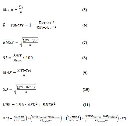
Based on the used statistical parameters, the higher R2 value will be more desirable, and the model with SI>0.3 will consider as bad performance, while 0.2 [
Results and Discussion
Relationship between independent parameters and compressive strength
LR model: Based on the statistical analysis using training and testing data below equation has been predicted with using 99 data as training data and 35 data as testing, with R2 equal to 0.73 for training data and 0.86 for testing data. RMSE value equal to 6.71 MPa for training data and 5.57 MPa for testing data, while MAE value is 5.55 MPa for training data and 4.63 MPa for testing data. OBJ value is equal to 7.44, and SI value in the range 0.2 to 0.3 which is showing good efficiency (Figure 13).
σp=57.04-25.96w/c+0.043C.C-0.032 S.C-0.03W.G+0.1*T

Figure 13: Linear regression model for training and testing data.
NLR model: With using 98 data as training data and 34 data as testing, the below equation has been predicted with R2 equal to 0.79 for training data and 0.89 for testing data. RMSE value equal to 5.92 MPa for training data and 4.76 MPa for testing data, while MAE value is 4.77 MPa for training data and 4.76 MPa for testing data. OBJ value is equal to 6.08, and SI value in the range 0.2 to 0.3 which is showing good efficiency (Figure 14).
σp=83.83-66.27w/b0.3+0.0034C.C1.66-0.00054S.C1.5-0.545W.G0.546 +7.3T0.246 (15)

Figure 14: Nonlinear regression model (plus form) for training and testing data.
MLR model: By using 98 data as training data and 35 data as testing, the below equation has been predicted with R2 equal to 0.73 for training data and 0.81 for testing data. RMSE value equal to 6.7 MPa for training data and 6.45 MPa for testing data, while MAE value is 5.642 MPa for training data and 5.488 MPa for testing data. OBJ value is equal to 7.8, and SI value in the range 0.2 to 0.3 which is showing good efficiency (Figure 15)
σp=1.79*(w/c-1.03) * (C.C0.258) * (T0.135)-(0.00017)*(w/c-5.38) * (C.C0.0286) * (W.G0.537) * (T0.0.001) (16)

Figure 15: MLR model for training and testing data.
ANN model: Based on the obtained analysis from ANN the following analysis have been obtained, and based on the value of RMSE, MAE and R2 the best reliable result has been chosen and the below graph obtained (Figure 16 and Table 3).
| No. of hidden layers | No. of neurons in left side | No. of neurons in right side | R2 | MAE (MPa) | RMSE (MPa) |
|---|---|---|---|---|---|
| 1 | 5 | 0 | 0.9819 | 1.8562 | 2.5517 |
| 1 | 6 | 0 | 0.9904 | 1.6862 | 2.2158 |
| 1 | 7 | 0 | 0.9911 | 1.5379 | 1.9477 |
| 1 | 8 | 0 | 0.9892 | 1.6136 | 2.0808 |
| 1 | 9 | 0 | 0.9865 | 1.6 | 2.1268 |
| 1 | 10 | 0 | 0.9913 | 1.3635 | 1.7758 |
| 1 | 11 | 0 | 0.9924 | 1.331 | 1.7552 |
| 1 | 12 | 0 | 0.9922 | 1.3055 | 1.723 |
| 2 | 4 | 4 | 0.9636 | 2.7497 | 3.6843 |
| 2 | 5 | 5 | 0.9842 | 1.9769 | 2.5085 |
| 2 | 6 | 6 | 0.9823 | 2.0118 | 2.4559 |
| 2 | 7 | 7 | 0.9807 | 2.2999 | 2.9697 |
| 2 | 8 | 8 | 0.9902 | 1.4929 | 1.9905 |
Table 3: Obtained results from trial and error by using ANN.

Figure 16: ANN model for training and testing data.
Models compression
Based on the obtained value of R2, MAE and RSME as in the figures below the ANN is most reliable compare to other proposed model when the value of R2 in ANN 26% higher than regression and 20% higher the NLR and 26% higher than MLR, value of RMSE in ANN 289% smaller than regression and 243% smaller the NLR and 288% smaller than MLR, value of MAE in ANN 327% higher than regression and 267% higher the NLR and 334% higher than MLR. OBJ value of ANN, lower than OBJ of LR by 418%, 323% of NLR and 443 % of MLR. SI value of ANN between 0 to 0.1, which performed excellency (Figures 17-21).

Figure 17: R2 value for three proposed models.

Figure 18: RMSE value for proposed models.

Figure 19: MAE value for proposed models.

Figure 20: OBJ value for proposed models.

Figure 21: SI value for proposed models.
Conclusion
Predicting an accurate and efficient statistical model to predict the compressive strength of the mortar, modified with waste material will be helpful, based on this process the following points have been obtained:
•Used range of waste glass as replacement of sand vary between 0 to 100%.
•With using different statistical parameters, R, RMSE, MAE, OBJ and SI showing that ANN is most accurate and efficient compare to other models since it provide higher value of R and lower value of other parameters.
•OBJ value of ANN lower than MAE of LR by 418%, 323% of NLR1 and 443 % of NLR.
•SI value of ANN between 0 to 0.1, which performed excellency.
•R value of ANN higher than R of LR by 26%, 20% of NLR1 and 26% of NLR.
•MAE value of ANN lower than MAE of LR by 327%, 267% of NLR1 and 334 % of NLR.
•RMSE value of ANN lower than RMSE of LR by 289%, 243% of NLR1 and 288% of NLR.
Funding
Not applicable.
Availability of The Data And Materials
All data generated or analysed during this study are included in this published article.
Conflict of Interest
We wish to confirm that there are no known conflicts of interest associated with this publication, and there has been no significant support for this work that could have influenced its outcome.
Research Involving Human Participants
This article does not contain ant studies involving animal’s human participants performed by any of the authors.
References
- Ling TC, Poon CS. Spent fluorescent lamp glass as a substitute for fine aggregate in cement mortar. J Clean Prod. 2017;161:646-654.
- Zeng JJ, Zhang XW, Chen GM, Wang XM, Jiang T. FRP-confined recycled glass aggregate concrete: Concept and axial compressive behavior. J Build Eng. 2020;30:101288.
- Ogundairo TO, Adegoke DD, Akinwumi II, Olofinnade OM. Sustainable use of recycled waste glass as an alternative material for building construction-A review. IOP Conf Ser: Mater Sci Eng. 2019;640(1):012073.
- Ling TC, Poon CS. Utilization of recycled glass derived from cathode ray tube glass as fine aggregate in cement mortar. J Hazard Mater. 2011;192(2):451-456.
[Crossref] [Google Scholar] [PubMed]
- Zhao H, Poon CS. A comparative study on the properties of the mortar with the cathode ray tube funnel glass sand at different treatment methods. Constr Build Mater. 2017;148:900-909.
- Ghafor K, Mahmood W, Qadir W, Mohammed A. Effect of particle size distribution of sand on mechanical properties of cement mortar modified with microsilica. ACI Mater J. 2020;117(1).
- Qadir W, Ghafor K, Mohammed A. Characterizing and modeling the mechanical properties of the cement mortar modified with fly ash for various water-to-cement ratios and curing times. Adv Civ Eng. 2019;2019(1):7013908.
- Ling TC, Poon CS, Lam WS, Chan TP, Fung KK. Utilization of recycled cathode ray tubes glass in cement mortar for X-ray radiation-shielding applications. J Hazard Mater. 2012;199-200:321-327.
[Crossref] [Google Scholar] [PubMed]
- Flores-Ales V, Alducin-Ochoa JM, Martin-del-Rio JJ, Torres-Gonzalez M, Jimenez-Bayarri V. Physical-mechanical behaviour and transformations at high temperature in a cement mortar with waste glass as aggregate. J Build Eng. 2020;29:101158.
- Cabrera-Covarrubias FG, Gomez-Soberon JM, Almaral-Sanchez JL, Arredondo-Rea SP, Mendivil-Escalante JM. Mechanical and basic deformation properties of mortar with recycled glass as a fine aggregate replacement. Int J Civ Eng. 2018;16:107-121.
- Choi SY, Choi YS, Yang EI. Effects of heavy weight waste glass recycled as fine aggregate on the mechanical properties of mortar specimens. Ann Nucl Energy. 2017;99:372-382.
- Corinaldesi V, Nardinocchi A, Donnini J. Reuse of recycled glass in mortar manufacturing. Eur J Environ Civ Eng. 2016;20(sup1):s140-s151.
- Guo MZ, Tu Z, Poon CS, Shi C. Improvement of properties of architectural mortars prepared with 100% recycled glass by CO2 curing. Constr Build Mater. 2018;179:138-150.
- Sikora P, Augustyniak A, Cendrowski K, Horszczaruk E, Rucinska T, Nawrotek P, et al. Characterization of mechanical and bactericidal properties of cement mortars containing waste glass aggregate and nanomaterials. Materials. 2016;9(8):701.
[Crossref] [Google Scholar] [PubMed]
- Yang S, Poon CS, Ling TC. Distribution of ASR gel in conventional wet-mix glass mortars and mechanically produced dry-mix glass blocks. Constr Build Mater. 2019;229:116916.
- Ahmad SA, Rafiq SK, Faraj RH. Evaluating the effect of waste glass granules on the fresh, mechanical properties and shear bond strength of sustainable cement mortar. Clean Techn Environ Policy. 2023;25:1989-2008.
- Rafiq SK. Modeling and statistical assessments to evaluate the effects of fly ash and silica fume on the mechanical properties of concrete at different strength ranges. J Build Pathol Rehabil. 2020;5:26.
- Fm Zain M, M Abd S. Multiple regression model for compressive strength prediction of high performance concrete. J Appl Sci. 2009;9(1):155-160.
- Ahmad SA, Ahmed HU, Ahmed DA, Hamah-ali BH, Faraj RH, Rafiq SK. Predicting concrete strength with waste glass using statistical evaluations, neural networks, and linear/nonlinear models. Asian J Civ Eng. 2023;24:3023-3035.
- Ahmad SA, Rafiq SK, Hilmi HD, Ahmed HU. Mathematical modeling techniques to predict the compressive strength of pervious concrete modified with waste glass powders. Asian J Civ Eng. 2024;25(1):773-785.
Citation: Ahmad SA, Abdulrahman AS, Ramezanianpour AM, Rafiq SK, Mahmood KOF, Jafer FS (2025) Modeling the Mechanical Properties of Sustainable Mortar Modified with Waste Glass Granular (Particles) Using Ann and Multi-Scale Approaches. Int J Waste Resour. 15:600.
Copyright: © 2025 Ahmad SA, et al. This is an open-access article distributed under the terms of the Creative Commons Attribution License, which permits unrestricted use, distribution, and reproduction in any medium, provided the original author and source are credited.