

Indexed In
- Open J Gate
- Genamics JournalSeek
- Academic Keys
- ResearchBible
- Cosmos IF
- Access to Global Online Research in Agriculture (AGORA)
- Electronic Journals Library
- RefSeek
- Directory of Research Journal Indexing (DRJI)
- Hamdard University
- EBSCO A-Z
- OCLC- WorldCat
- Scholarsteer
- SWB online catalog
- Virtual Library of Biology (vifabio)
- Publons
- Geneva Foundation for Medical Education and Research
- Euro Pub
- Google Scholar
Useful Links
Share This Page
Journal Flyer

Open Access Journals
- Agri and Aquaculture
- Biochemistry
- Bioinformatics & Systems Biology
- Business & Management
- Chemistry
- Clinical Sciences
- Engineering
- Food & Nutrition
- General Science
- Genetics & Molecular Biology
- Immunology & Microbiology
- Medical Sciences
- Neuroscience & Psychology
- Nursing & Health Care
- Pharmaceutical Sciences
Research Article - (2023) Volume 12, Issue 2
Explainable Convolutional Neural Network Based Tree Species Classification Using Multispectral Images from an Unmanned Aerial Vehicle
Ling-Wei Chen, Pin-Hui Lee and Yueh-Min Huang*Received: 30-Dec-2022, Manuscript No. AGT-23-19501; Editor assigned: 02-Jan-2023, Pre QC No. AGT-23-19501 (PQ); Reviewed: 16-Jan-2023, QC No. AGT-23-19501; Revised: 21-Mar-2023, Manuscript No. AGT-23-19501 (R); Published: 28-Mar-2023, DOI: 10.35248/2168-9891.23.12.310
Abstract
We seek to address labor shortages, in particular, the aging workforce of rural areas and thus facilitate agricultural management. The movement and operation of agricultural equipment in Taiwan is complicated by the fact that many commercial crops in Taiwan are planted on hillsides. For mixed crops in such sloped farming areas, the identification of tree species aids in agricultural management and reduces the labor needed for farming operations. General optical images collected by visible-light cameras are sufficient for recording but yield suboptimal results in tree species identification. Using a multispectral camera makes it possible to identify plants based on their spectral responses. We present a method for tree species classification using UAV visible light and multispectral imagery. We leverage the differences in spectral reflectance values between tree species and use near infrared band images to improve the model’s classification performance. CNN based deep neural models are widely used and yield highaccuracies, but 100% correct results are difficult to achieve, and model complexity generally increases with performance. This leads to uncertainty about the system’s final decisions. Interpretable AI extracts key information and interprets it to yield a better understanding of the model’s conclusions or actions.We use visualization(four pixel level attribution methods and one region level attribution method) to interpret the model post-hoc. Fuzzy IG for pixel level attribution best represents texture features, and region level attribution represents life regions more effectively than pixel level attribution, which aids human understanding.
Keywords
Explainable AI (XAI); Convolutional Neural Network (CNN); Multispectral; Tree species classification; Unmanned Aerial Vehicle (UAV)
Introduction
Taiwan's land is narrow and densely populated, and hillside land comprises over 70% of the country's total land area. It contains rich natural resources, and there are more than 30 kinds of fruits, with production areas all over the country. Constrained by the steep terrain of Taiwan's sloping land, which is not conducive to the movement and operation of equipment, agricultural work is still mainly carried out manually, which is laborious and time consuming. In addition, many sloping plots of land are planted with mixed fruit trees, which adds difficulty to planting operations. Species investigation is particularly important for these reasons. Because traditional manual survey work is time consuming and labor intensive, methods have been developed for automated tree species through smart agriculture, which not only yields a better understanding of the distribution of tree species on farmland but also provides effective geographical environment information that facilitates the implementation of pest control and pesticide spraying operations [1].
In practice, smart agriculture requires various Artificial Internet of Things (AIoT) and smart agricultural machinery or technologies, for instance, automated environmental control equipment, sensors, Artificial Intelligence (AI), agricultural robots, and agricultural drones. Using technologies such as Unmanned Aerial Vehicles (UAVs) and deep learning, data analysis can improve agricultural management and reduce agricultural labor requirements. In recent years, UAVs have greatly improved the efficiency of agricultural production and enabled production in a more immediate, lower cost, and less labor-intensive way. In tasks such as forest management, environmental monitoring and crop identification, UAVs are often equipped with cameras for image collection. Although general high resolution lenses in the visible light band are sufficient to meet the needs of recording, in agricultural applications, to obtain more effective information for precision agriculture, it is necessary to integrate additional components such as multispectral sensors, hyperspectral sensors, or thermal imaging sensors [2].
With the increasing ubiquity of AI come questions of trust, bias, accountability, and process, all concerning how the machines are reaching their conclusions. AI based systems are not 100% perfect, and improvements in system performance are often achieved by increasing model complexity, making these systems a “black box” and leading to uncertainty about how they operate and how they ultimately make decisions. Thus, insights into decisions not only elicit trust but also prevent life threatening mistakes [3]. Explainable AI research delves deeper into the black box of deep learning and yields information or explanations about how an algorithm has come to its conclusions or actions. In addition to providing accountability, XAI can be useful for system fine-tuning.
For these reasons, we attempt to use a UAV with multi-spectral sensors and XAI technology to automatically identify and investigate mixed crops in sloped farming areas, reducing costs and labor burdens and yielding useful information for agricultural management. This facilitates follow-up pest management and pesticide spraying operations and increases the transparency of deep learning models. We use post-hoc explanation methods in XAI four pixel level attribution methods and one regional level attribution method-to visualize important model learning features to better understand the model’s decision factors for use in revising the model. The experimental results show that regional attribution combines pixel level attribution and image over-segmentation to rank block importance to more effectively quantify feature meaning and importance.
Materials and Methods
Telemetry image monitoring
In the remote sensing of vegetation, research data is most often obtained in the form of field surveys or observations [4]. However, the amount of information for field surveys is usually limited because such surveys involve considerable transportation, equipment, and labor costs. For study of the natural environment in particular, factors such as climate and topography also limit the sampling frequency. Remote sensing monitoring is a popular topic for research on precision agriculture, forestry management, crop yield prediction, irrigation, weed detection, and so on. Platforms include satellites, UAVs, and Unmanned Ground Vehicles (UGVs).
Challenges of remote vegetation sensing include increasing data volumes and computational loads and more diverse data structures, whose dimensions (spatial, temporal, and spectral) often are characterized by complex relationships. Therefore, using remote sensing data for vegetation assessment and monitoring requires efficient, accurate, and flexible analytical methods. Over the past few decades, various technological advances have increased the availability of remote sensing data.
Multispectral UAV imagery
To date, remote sensing research relies primarily on satellites or aircraft. In the past, multispectral satellites were the focus of attention: They are low cost and cover large areas, helping to map forest or vegetation cover types [5]. The disadvantages of such satellites are their low resolution, which makes it difficult to identify tree species and support precision agriculture. After 2000, many studies began to use data from commercial satellites in the form of high-resolution panchromatic and multi-spectral images for tree species classification. In addition, recent studies using drones have successfully classified tree species using images with resolutions ranging from 0.2 to 3.0 meters. Novel remote sensing platforms such as microsatellite swarms or UAVs yield imagery of vegetation canopies with increased spatial detail.
UAVs have been used experimentally in forestry applications over the past few decades [6]. Compared to manned aircraft, drones are an easy to use, low-cost telemetry tool. In addition, drones can fly near tree canopies to capture extremely high resolution images. Most related studies use special hardware such as visible light cameras, multispectral sensors, hyperspectral sensors, and Light Detection and Ranging (LIDAR) sensors to achieve good results when classifying tree species [7]. Visible light imagery can also be used in combination with Near Infrared (NIR) or multi-spectral imagery to improve the accuracy of biomass calculations [8]. Applications also exist that combine multi-spectral or hyperspectral sensors and lidar data; although this method of data acquisition yields superior performance, the sensing equipment involved is expensive [9].
Vegetation telemetry technology and AI
Neural network [10] technology has been under development for over three decades and is now a dominant approach. Support vector machines were popular from 1980 to 2000, primarily because few neural network layers (about 1 to 3 layers) could be built at that time, resulting in a limited number of features that the networks could learn and thus poor model performance; these are termed shallow neural networks. Inspired by human learning, Artificial Neural Networks (ANNs) employ connected units to learn features from data. In recent years, with the improvement of various aspects of computer technology, it has become much easier to build larger neural networks, which has led to major efficiency breakthroughs in deep neural networks, such that neural networks are once again superior to previous methods. Deep learning models, or deep ANNs with more than two hidden layers, are complex enough to learn features from data, removing the need to manually extract features based on human experience and prior knowledge.
CNN based deep neural models have achieved unprecedented breakthroughs in computer vision tasks and are one of the most successful network architectures for methods ranging from image classification, object detection, and semantic segmentation to image captioning, visual question answering, and most recently visual dialog [11].
Deep learning, a breakthrough technology, has been used for data mining and remote sensing research. Research that combines deep learning and remote sensing data has shown great potential in plant detection, forest cover mapping, and crop damage assessment. One advantage of deep learning over Machine Learning (ML) methods is that it does not require manual feature extraction. An ML method extracts texture features, vegetation indexes, and original band values, after which hyperspectral data can be used for feature selection to reduce dimensionality and avoid the “curse of dimensionality” and high computational costs caused by high dimensional spaces [12]. Deep learning exploits complete feature information, especially information related to spatial pixel relationships such as tree texture and shape. Therefore, even with simple digital images, deep learning can yield high detail and high accuracy recognition results.
Deep learning has become an important tool for agricultural classification and quality control due to its powerful and fast feature extraction capabilities. Applications use deep learning and imagery to assist agriculture for tasks such as grape variety classification using visible light imagery with AlexNet and Mask R-CNN; crop identification and land use classification using multispectral satellite imagery; crop classification using six CNN architectures trained on 14 classes of multi-spectral land cover imagery; plant disease detection using the VGG-16 model; weed detection in sugar beet fields using VGG-16 and classification of field land cover using the Inception-v3 model [13].
Explainable AI
As AI becomes more ubiquitous, questions of trust, bias, accountability, and process become more important: How exactly are these machines reaching their conclusions? AI based systems are not 100% perfect, and improvements in system performance are usually achieved by increasing model complexity, making these systems a “black box” and leading to uncertainty about how they operate and how they ultimately make decisions. Thus, insights into decision making not only elicit trust but can also prevent life-threatening mistakes [14].
Explainable AI research aims to peek into the black box of ML and deep learning and extract information or explanations for how an algorithm has come to certain conclusions or why it has taken certain actions. In addition to accountability, XAI can assist in tuning machine learning systems. The inputs and outputs of ML algorithms as well as their network design are still determined by humans and are therefore often subject to human error or bias. XAI addresses these issues, providing end users with greater confidence and increasing trust in ML systems.
In practical situations, linear models or shallow neural networks are often not expressive enough to make predictions. As a result, deep neural networks are gradually taking over as the most common predictive model. Depending on the neural network architecture, a single prediction can involve millions of mathematical operations. Humans must consider millions of weights interacting in complex ways to understand the predictions of neural network models. The complexity of deep neural network models greatly complicates model interpretation, making it necessary to develop specific interpretation methods to explain the behavior and predictions of the model.
Given the opaque nature of neural network systems such as CNNs, it is difficult to ascertain which layers or parameters affect the training process. In this study, we focus not on how the model learns but rather on understanding what features have the greatest effect on the model in an effort to increase model reliability and make the models more transparent.
Research architecture
In this section we introduce the system architecture, neural network framework, and image classification performance indices.
System architecture: The system architecture of this study is shown in Figure 1. First, we placed Ground Control Points (GCPs) in the experimental area to correct the threedimensional coordinates. Next, we collected images of the experimental site through a visible light lens and an onboard multispectral lens. After this came orthophoto production, data preprocessing, training classification model, and explainable AI.

Figure 1: System architecture.
Production of orthophoto images requires multi-spectral radiometric calibration to reduce light caused radiation effects. To accurately match the visible light image and the multi-spectral image, we used GIS software to inspect the coordinates of the fixed feature points and correct the coordinates. The processing steps are shown in Figure 2. After completing these operations, we proceeded to the data preprocessing stage.

Figure 2: Orthophoto production.
For image preprocessing, we resampled the multi-spectral orthophoto via bicubic interpolation to the same size and resolution as the visible light orthophoto. Next, we used a sliding window to cut the orthophoto image into smaller sub images, of which 20% were taken as the dataset, which we further classified manually. This dataset was then partitioned into 80% for the training set and 20% for the testing set, as shown in Figure 3.

Figure 3: Data preprocessing.
The model training steps are shown in Figure 4. We input the training set to the VGG-16 model, adjusted the parameters, trained the model, and then evaluated the model performance on the test set. If the evaluation indices did not meet our expectations, we adjusted the parameters and re-trained the model; if this then met our expectations, we considered this the best model. We used the best model to classify the sub images over the whole area, and present the classification results as a multicolor distribution map.

Figure 4: Model training.
Last, in the XAI stage, we used four pixel level attribution methods to visualize features, and used a region level attribution XRAI method to better understand the reason for the model's decisions.
Below, we describe the neural network model and the image classification metrics for the experiments, and present the results of the study.
Neural network framework: We extended the experimental content for this study from our previous tree species classification study in which we compared the performance of four CNN architectures on visible light images CNN-4, VGG-16, VGG-19 and ResNet-50 of which the VGG-16 model yielded the highest overall accuracy rate (0.852). Therefore, in this study we used a modified VGG-16 model with an added multispectral NIR band to improve classification accuracy, and added post-hoc back propagation gradient based explanation methods to produce feature attributions.
The modified VGG-16 model is shown in Figure 5. Taking the model architecture used in the Dongshan area as an example, the input image size is 224 × 224 × 3, and the model includes 13 convolution layers, 5 max pooling layers, and 3 fully connected layers. To better understand which features have the greatest effect on the classification results, we calculated and generated an attribution map of the image via gradient backpropagation.

Figure 5: Explainable VGG-16 network.
Performance indices: After training a model, we evaluate the model’s performance. Many validation indices can be used as performance indicators. In this study, we used a neural network model for multiclass image classification of a variety of tree species, buildings, and roads in the experimental area (Table 1). To evaluate the performance of the models, we use the confusion matrix, the overall precision rate, and the recall rate.
| Predicted positive | Predicted negative | |
|---|---|---|
| Actual positive | True Positive (TP) | False Positive (FP) |
| Actual negative | False Negative (FN) | True Negative (TN) |
Table 1: Binary confusion matrix.
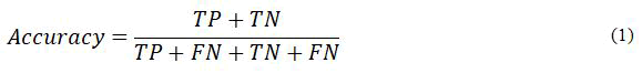
A confusion matrix, a standard format for evaluating models, has N rows and N columns. Each column represents the predicted value, and each row represents the actual value. The matrix shows whether there is confusion between multiple categories, that is, how many results the model has judged correctly and how many results are wrong. From the confusion matrix we calculate metrics such as accuracy, precision, recall, and F-score. For binary classification, the confusion matrix has 2 rows and 2 columns, as shown in Table 1. Naturally, we seek to maximize true positives and true negatives while minimizing false positives and false negatives, which are respectively termed type I errors and type II errors.
Overall accuracy, a common metric for model performance, is calculated using formula 1, which calculates the correct ratio of all predictions and describes the ability of the model to find the correct class. However, note that accuracy considers each class to be equal.
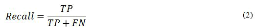
Recall, also known as the true positive rate or the hit rate, indicates how many true positive samples were correctly classified; see formula 2.
Experimental data
This section introduces the experimental site, GCP placement and measurement, orthophoto production, feature point matching, and data preprocessing. Orthophoto production includes radiometric calibration. Data preprocessing includes multispectral image resampling and dataset creation via cropping, classification, data augmentation, and data balancing.
Experimental site
Considering the difficulty of farming and the complexity of planting types due to the sloped terrain, we chose an experimental site in Dongshan, specifically Dongshan district, Tainan city, Taiwan. The terrain slopes downward from the northeast to the west. The main crops at the site are longan, plantain, jujube, avocado, and Rutaceae trees. With this study we seek to reduce the inconvenience of farming by automatically identifying tree species in the field using UAVs and AI. However, as the site is surrounded by mountains, communication signals are easily interrupted, which hinders signal transmission and reception during measurement operations, increasing the difficulty of this study.
Ground control point placement and measurement
In this study, after we placed Ground Control Points (GCPs) at the site to facilitate accurate orthophotography, we flew a quadrotor UAV equipped with a visible light camera and a multi-spectral camera back and forth at a high altitude to scan the site and capture imagery at an angle perpendicular to the ground.
GCPs are a common way to improve the geographic accuracy of map surveying, and greatly impact the construction of Digital Terrain Models (DTMs). When placing control points, considerations include their number, spacing, and locations.
In this study, ten square marks were drawn with white paint on open and flat ground at the Nanhua experimental site. The center points of these squares were measured using a handheld satellite locator (stonex P9A) and a geodesic GNSS receiver (stonex S3A), and the three-dimensional geographic information for each point was recorded. When creating an orthophoto, the coordinates of each control point were imported to produce orthophoto with accurate coordinates.
Orthophoto production
In this study, visible light photos and multi-spectral photos were used to obtain orthophotos of the complete area via geometric correction and image mosaics. Radiometric correction was used on the multi-spectral photos to eliminate image distortion caused by radiometric errors. Given these orthophotos, subsequent experimental steps were carried out for the visible light orthophotos and multi-spectral orthophotos.
We captured aerial imagery of the site using the drone and obtained geographic information about the real surface according to the Digital Elevation Model (DEM) of the site; the drone was flown at a height of 30 meters above ground. The process of making orthophotos is shown in Figure 6. Equipped with a visible light optical lens and a multi-spectral optical lens, the UAV scanned the site to capture high altitude imagery. We imported the individual images into Pix4Dmapper, set the parameters and output specifications, calibrated the site’s ten ground control points, and produced a high-altitude orthophoto covering the entire area. To correct spatial dislocations or distortions during image stitching, we input the spatial geographic information (longitude, latitude, and altitude) of the control points into Pix4Dmapper and aligned all control points with the correct three-dimensional coordinates to reduce aerial measurement error.

Figure 6: Orthophoto production process.
The five high altitude images used in this study were captured on January 14, March 19, April 10, June 16, and July 18, 2022. Each image is the product of one visible light orthophoto and five multi-spectral orthophotos, including the red, green, blue, NIR, and red-edge spectra. Although the spatial resolution of the multi-spectral images was lower than that of the optical images, the multi-spectral images contain five channels of rich multiple-spectral reflectance information.
Radiometric calibration: Image data is laid out as a large matrix of numbers, where each pixel in the image is a number that corresponds to the intensity of radiation at a certain wavelength. This allows us to see objects such as buildings, roads, and grass in the imagery. However, these pixel values also reflect any environmental conditions present when the data was collected, such as changes in lighting in the form of sunny and cloudy days, sun orientation, intermittent cloud cover, and so on.
Since plant reflectance can be used as an indicator of a plant’s health, disease problems, or different species, accurate reflectance values are essential for understanding plant physiology and comparing image changes over time and space. Without high quality radiometric calibrations, the effects of lighting conditions cannot be taken into account, which greatly complicates time based analysis [15].
We adopted a Corrected Reflective Panel (CRP), a radiometric calibration method common to telemetry applications which is the most commonly used method historically. As the panel has pre-measured reflectance values, it can be used as a control reference. To use it, we take a photo of the corrected reflectance panel, which allows us to assign known reflectance values to the panel's pixels and adjust the rest of the dataset accordingly. The Pix4Dmapper software calculates the reflection values from the image of the corrected reflective panel as a benchmark to correct orthophoto data.
Feature point matching
To improve tree species identification using spectral information, we sought to combine visible light orthophotos and multi-spectral orthophotos. The reflectance values of near infrared light vary greatly among plants, and can thus be used to differentiate tree species; accordingly, we used NIR channel multispectral images for these experiments.
When constructing orthophoto images, we imported the coordinates of the ten control points to produce the most accurate output. However, there were still slight errors in the coordinate space attached to the two images.
To correct these errors, we first imported the visible light orthophoto and the multi-spectral orthophoto into the global mapper, recorded the error of the center coordinates of each control point, and took the average as the overall deviation value, including the horizontal and vertical offsets. Then, we modified the TIFF world file (TFW) file corresponding to the orthophoto with the overall deviation value to correct the deviation in the two images. TFW is a space parameter description file with six columns of content for TIFF files, and can be opened and edited using a general ASCII text editor. The first column represents the pixel resolution in the X direction (row), the second column represents the X-axis rotation amount, the third column represents the Y-axis rotation amount, the fourth column represents the pixel resolution in the Y direction (column), and the sixth and seventh columns represent the X and Y geographic coordinates of the upper left pixels respectively; thus we used the corrections in the sixth and seventh columns.
Data preprocessing
Here we describe the image preprocessing needed for model training, including the multi-spectral orthophoto re-sampling and the processing of the dataset samples, which involved cutting, classification, image data enhancement, and data balancing preprocessing, as described in the following subsections.
Multi-spectral image re-sampling: We collected five aerial images of the Dongshan site in 2022, and used software to produce five date aerial orthophotos as a combination of visible light orthophotos and multi-spectral orthophotos (five channels). We used re-sampling to increase the resolution of the multispectral orthophotos to match the visible light images.
Take the orthophoto taken on March 19 as an example: The resolution of the visible light orthophoto was 0.85 cm/pixel, and that of the multi-spectral orthophoto was 1.39 cm/pixel. To produce a sub-image that covers an area of 85 × 85 square centimeters, the visible light orthophoto would need to be cropped to 100 × 100 pixels, and the multi-spectral image would need to be 61 × 61 pixels. We used bicubic interpolation re-sampling to increase the size of the multispectral images so that the two images would have the same coverage and size for image fitting and conform to the format of the input model.
Dataset classification
This section describes the steps taken to create the dataset. The orthophotos covering the experimental site were cropped to fit and 20% of the resultant subimages were selected as the training set and manually classified into several categories.
Image cropping: Since the purpose of this study is to identify tree species at the experimental site using the VGG-16 model, we cropped the orthophoto images to fit and used 20% of the resultant subimages as the dataset, of which 80% and 20% were used as the training set and the testing set, respectively. Note that as the canopy area of different crops at the site differed, there was no one window size that would fit all crops. Empirically, we determined the most suitable window size to be 100 × 100 pixels, as this captured local crop features and cut out unnecessary information. As larger viewports contained multiple crops or targets, we chose as small a viewport size as possible, but not so small that it contained too few features. To ensure that the images covered enough local features, we cropped the Dongshan orthophoto into 32 × 32 pixel image patches.
Classification: After cropping, the subimages were classified manually. Crops at the site included longan, plantain, jujube, avocado, and rutaceae, among which longan is the subject of this study. The categories were set to longan, other trees, soil/roads, and buildings, for a total of four categories, as shown in Figure 7.

Figure 7: Dataset classes.
Image data augmentation: Data augmentation is common in image processing. Data imbalance is a common problem with image recognition; it is difficult to train a good neural network when there are too few images of a certain class, or when there is insufficient data in general. In this case we augment the data to increase the amount of data using physical techniques such as flipping the image, adjusting the lightness and darkness, adjusting the scale, and panning, all of which produce new images. Note that for humans, these are the same images, but for the machine, these are new images.
We sought to increase the amount of data by horizontal flipping and vertical flipping. After flipping, there was still not enough data, so we further adjusted the lightness and darkness to increase the amount of data. For example, the building in Table 2 had only 182 original images; adding horizontal and vertical flips yielded a total of 546 images, and then producing three shades of each of the 152 original images yielded another 456 images, for a total of 1,002 images, which we manually adjusted down to 1,000 images.
| Class | Original data size | Data size after augmentation |
|---|---|---|
| Longan | 2,047 | 1,000 |
| Other trees | 1,314 | 1,000 |
| Soil and roads | 974 | 1,000 |
| Architecture | 182 | 1,000 |
| Total | 4,517 | 4,000 |
Table 2: Training data sizes.
Results and Discussion
Here we describe the classification model for the Dongshan site, present the tree species classification results, and provide the post-mortem explanation of the model. In this study, we use four post-hoc explanation methods based on gradient back propagation: A saliency map, Integrated Gradients (IG), guided IG, and blur IG; pixel level attribution is also used to visualize features. We also compare pixel level attribution in terms of IG.
Classification model and results
This study was conducted using visible-light and multi-spectral orthophotos of the Dongshan site taken on January 20, 2022. Here we classify the various crops into tree species, and discuss the experimental results.
Classification model: In this experiment, the visible light orthophotos and multi-spectral NIR orthophotos were used to classify the tree species of various crops at the site. The main tree species at the site were longan, bananas, jujube, avocado, and rutaceae. As the longan were in the differentiation period, their canopies were generally green in appearance. However, as there were fewer crop species and no litchi trees at the site, and the planting pattern was less complex, there were significant differences in the characteristics of each tree.
Table 3 shows the training parameters (learning rate, batch size, and training epochs), training time, and performance evaluation metrics (overall accuracy and recall) of the model. To avoid overfitting, the learning rate and batch size were selected using the early-stop strategy.
| Imagery date | January 20, 2022 |
|---|---|
| Model | VGG-16 |
| Channel selection | Visible+Multispectral NIR |
| Training parameters | |
| Learning rate | 0.00001 |
| Batch size | 64 |
| Training epochs | 175 |
| Training time | 181 seconds |
| Evaluation metrics | |
| Overall Accuracy (OA) | 0.878 |
| Recall | R(0)=0.880 |
| R(1)=0.815 | |
| R(2)=0.980 | |
| R(3)=0.837 | |
Table 3: Training parameters, training time, and evaluation indices.
Classification results: On January 20, 2022, when the aerial imagery was captured, the longan was differentiating and the canopy appearance was dominated by green leaves. The crops at this site are simple with a relatively consistent planting pattern, which facilitates tree species identification. The recall rate of all four categories (longan, other trees, soil/road, and buildings) was over 80%. After excluding soil/roads, the highest recall rate was 0.88 for longan: The model achieved good recognition performance for longan trees.
Figure 8 shows the recognition results. The left image is the visible-light orthophoto of the site; the right image is the distribution map of the recognition results, with different colors for each class, which clearly shows the location and types of the various crops.

Figure 8: Distribution map of recognized tree species.
Post-hoc model explanations
This study uses AI visualization methods for important features to yield a better understanding of the factors considered by the model for decision making. Visualization can be accomplished at the pixel level as well as the region level. Here we compare four gradient based backpropagation methods using pixel level attribution and then compare pixel level attribution with region based attribution.
Post-hoc explanations using pixel level attribution: Four pixel level attribution methods were used for the model: Saliency map, Integrated Gradients (IG), guided Integrated Gradients (guided IG), and blur Integrated Gradients (blur IG). IG, guided IG, and blur IG present input features that have the most influence on the predicted category as grayscale images in which brighter pixels are more important.
• A saliency map represents pixel level importance with respect
to a classification category by the gradient magnitude,
visualized as an attribution map.
• IG solves the problem of gradient saturation generated by the
saliency map: The gradient’s integral value is used as the
importance for the attribution map to reveal more effective
information. However, as IG can generate noise outside
relevant regions, the following methods 3 and 4 are used to
eliminate noise.
• Guided IG uses adaptive paths to improve IG by dynamically
adjusting the model’s attribution path, which reduces noise by
moving in the direction of the lowest correlation bias.
• Blur IG uses Gaussian filtering and the Laplacians of
Gaussians (LOG) operator for edge detection, which produces
understandable attributions and reduces noise to highlight
more highly correlated pixels.
Figure 9 shows the attribution diagrams obtained from the four pixel level attribution methods. Brighter pixels have a greater influence on model prediction. From this figure, the following three points can be summarized.
Saliency map vs. component gradient: As the saliency map calculates the attribution gradient, when the gradient of a pixel with a classification score close to 1 is close to 0, it cannot effectively represent these important pixels. The IG attribution map highlights more important regions than the saliency map because it uses gradient scores instead of gradients, which presents important pixels in the attribution map.
Integral gradient vs. guided IG vs. blur IG: The guided IG and blur IG methods both reduce noise in IG. Blur IG is most effective in clearly presenting edge textures and reducing noise, and is thus easier to understand. We observe poor results for guided IG. This study suggests that IG facilitates a better understanding of where the important pixels are.
Correct classification vs. misclassification: The results of the four pixel level attribution methods for the two correctly classified images show that the model mainly uses the pixels at the edge of the lobster bush to differentiate the category. For the two misclassified images, the model extracts not only features of the dragon's eye but also soil pixels on the side as its important features; the blur IG attribution map shows that the small scale granular textures are seen to be important, in contrast to correctly classified large scale bush textures, thus explaining the misclassification.

Figure 9: Post-hoc explanation methods using pixel level attribution.
Explanation with Ranked Area Integrals (XRAI): Explanation with Ranked Area Integrals (XRAI), an IG based area level attribution method combined with over segmented image processing technology, iteratively calculates the integral value of the gradient [16-19]. Area importance is used to merge smaller areas into larger areas by predicting whether a certain block is a positively affected image area according to pixel level information in the area. Figure 10 shows the relationship between XRAI and other types of pixel level attribution [20].
Figure 10: Pixel level attribution vs. XRAI.
Pixel level attribution vs. XRAI: In this section, we compare IG based pixel level attribution with XRAI for area attribution.
Pixel level attribution provides attribution of fine texture to the image model by attributing to a single pixel. However, in this method significant pixels may be scattered throughout the image, which makes it difficult to understand and interpret. XRAI calculates significance at the area level rather than the pixel level by combining IG pixel level attribution and oversegmentation. The resulting areas are ranked to present the top 30% of the highest importance.
Figure 2 compares the two attribution methods for correct and incorrect lobotomies. In the XRAI heat map, yellow indicates more important areas and indigo indicates less important areas.
We have two observations for this figure.
• XRAI presents importance as a regional heat map and masks
areas outside the top 30% of the most important ones. This
makes it easier than pixel level attribution to understand
features that have a greater influence on the model.
• With XRAI, it is clear that the key longan features are the
borders between clumps of leaves; images are misclassified
because the important feature areas are on the border between
trees and weeds.
Figure 11 compares the attribution methods for the other three categories. We observe that the important feature of other trees is the long stripes of their leaves; that because soil and roads have fewer textural features, the most important feature is the darker areas and the most important feature of buildings is their dark, regular texture (Figure 12).

Figure 11: Attribution methods with correctly classified and misclassified longan.

Figure 12: Attribution methods with correctly classified nonlongan trees, soil roads, and buildings.
Conclusion
In this study, we propose a method for tree species identification that combines visible light and multi-spectral NIR. We locate and survey the experimental site, collect the drone images, and produce and calibrate the optical and multispectral images to train the identification model and present a distribution map of the tree species classification results. In addition, we use various visualization methods to interpret the model post-hoc in order to understand the factors that play into the model’s decisions: Four pixel level attribution methods (saliency map, IG, guided IG, blur IG) and one area attribution method (XRAI).
Of the pixel level attribution methods, IG improves the gradient saturation problem of the saliency map, and guided IG and blur IG improves reduce the noise of IG. The experimental results show that the attribution map of blur IG presents the texture features that are most easily understood by humans. Between pixel attribution and IG based XRAI area attribution, the latter presents the importance of blocks in the form of area and heatmaps, and shows the top 30% important parts after ranking each area, which makes the visualization easier to understand.
Author Contributions
The contributions of this study are as follows:
• We map the distribution of crop species on arable land over
large areas, undulating, or difficult to manage topography. The
method clearly distinguishes the distribution of various tree
species, which facilitates farming and arable land management
and provides information on the geographic environment and
tree species for future development of smart agriculture.
• The proposed interpretable multi-spectral tree species
identification process uses visible light optical
images combined with multi-spectral NIR images to
provide additional spectral information for the model to
learn from; this enhances the model's identification effect
compared with the use of visible light images alone.
• The visualization approach yields a better understanding of
the model’s decision making process and facilitates
more timely model adjustments. It makes the model
more transparent and provides insight into the model to
determine whether the model is learning in the right
direction. We compare various visualization methods as a
reference for future research in the field of deep learning.
References
- Tetila EC, Machado BB, Astolfi G, de Souza Belete NA, Amorim WP, Roel AR, et al. Detection and classification of soybean pests using deep learning with UAV images. Comput Electron Agric. 2020;179:105836.
- Pally RJ, Samadi S. Application of image processing and convolutional neural networks for flood image classification and semantic segmentation. Environ Modell Softw. 2022;148:105285.
- Pandey A, Jain K. An intelligent system for crop identification and classification from UAV images using conjugated dense convolutional neural network. Comput Electron Agric. 2022;192:106543.
- Adadi A, Berrada M. Peeking inside the black-box: A survey on Explainable Artificial Intelligence (XAI). IEEE access. 2018;6:52138-52160.
- Fassnacht FE, Latifi H, Sterenczak K, Modzelewska A, Lefsky M, Waser LT, et al. Review of studies on tree species classification from remotely sensed data. Remote Sens Environ. 2016;186:64-87.
- Salovaara KJ, Thessler S, Malik RN, Tuomisto H. Classification of Amazonian primary rain forest vegetation using landsat ETM plus satellite imagery. Remote Sens Environ. 2005;97(1):39-51.
- Whyte A, Ferentinos KP, Petropoulos GP. A new synergistic approach for monitoring wetlands using sentinels-1 and 2 data with object-based machine learning algorithms. Environ Modell Softw. 2018;104:40-54.
- Khaliq A, Comba L, Biglia A, Ricauda Aimonino D, Chiaberge M, Gay P. Comparison of satellite and UAV based multispectral imagery for vineyard variability assessment. Remote Sens. 2019;11(4):436.
- Goodbody TRH, Coops NC, Marshall PL, Tompalski P, Crawford P. Unmanned aerial systems for precision forest inventory purposes: A review and case study. For Chron. 2017;93(1):71-81.
- Iizuka K, Yonehara T, Itoh M, Kosugi Y. Estimating tree height and Diameter at Breast Height (DBH) from digital surface models and orthophotos obtained with an unmanned aerial system for a Japanese cypress (Chamaecyparis obtusa) forest. Remote Sens. 2017;10(1):13.
- Mlambo R, Woodhouse IH, Gerard F, Anderson K. Structure from Motion (SfM) photogrammetry with drone data: A low cost method for monitoring greenhouse gas emissions from forests in developing countries. Forests. 2017;8(3):68.
- Paneque-Galvez J, McCall MK, Napoletano BM, Wich SA, Koh LP. Small drones for community-based forest monitoring: An Assessment of their feasibility and potential in tropical areas. Forests. 2014;5(6):1481-1507.
- Dalponte M, Bruzzone L, Gianelle D. Tree species classification in the Southern Alps based on the fusion of very high geometrical resolution multi-spectral/hyperspectral images and LiDAR data. Remote Sens Environ. 2012;123:258-270.
- Franklin SE, Hall RJ, Moskal LM, Maudie AJ, Lavigne MB. Incorporating texture into classification of forest species composition from airborne multi-spectral images. Int J Remote Sens. 2000;21(1)61-79.
- Ozdemir I, Karnieli A. Predicting forest structural parameters using the image texture derived from worldview 2 multispectral imagery in a dryland forest, Israel. Int J Appl Earth Obs Geoinf. 2011;13(5):701-710.
- Shen X, Cao L. Tree species classification in subtropical forests using airborne hyperspectral and LiDAR data. Remote Sens. 2017;9(11):1180.
- Kanungo T, Mount DM, Netanyahu NS, Piatko CD, Silverman R, Wu AY. An efficient k-means clustering algorithm: Analysis and implementation. IEEE Trans Pattern Anal Mach Intell. 2002;24(7):881-892.
- Li G, Han WT, Huang SJ, Ma W, Ma Q, Cui X. Extraction of sunflower lodging information based on UAV multi-spectral remote sensing and deep learning. Remote Sens. 2021;13(14):2721.
- Alonzo M, Bookhagen B, Roberts DA. Urban tree species mapping using hyperspectral and lidar data fusion. Remote Sens Environ. 2014;148:70-83.
- Ke YH, Quackenbush LJ, Im J. Synergistic use of quickbird multispectral imagery and LIDAR data for object based forest species classification. Remote Sens Environ. 2010;114(6):1141-1154.
Citation: Chen L, Lee P, Huang Y (2023) Explainable Convolutional Neural Network-Based Tree Species Classification Using Multispectral Images from an Unmanned Aerial Vehicle. Agrotechnology. 12:310.