

Indexed In
- Open J Gate
- RefSeek
- Hamdard University
- EBSCO A-Z
- OCLC- WorldCat
- Publons
- International Scientific Indexing
- Euro Pub
- Google Scholar
Useful Links
Share This Page
Journal Flyer
Open Access Journals
- Agri and Aquaculture
- Biochemistry
- Bioinformatics & Systems Biology
- Business & Management
- Chemistry
- Clinical Sciences
- Engineering
- Food & Nutrition
- General Science
- Genetics & Molecular Biology
- Immunology & Microbiology
- Medical Sciences
- Neuroscience & Psychology
- Nursing & Health Care
- Pharmaceutical Sciences
Review Article - (2025) Volume 14, Issue 2
Quantifying Carbon Sequestration of Forest Ecosystem Using GIS and Remote Sensing: The Case of Yeraba State Forest East Gojjam Zone Amhara Regional State
Tilahun Abie Fetene*Received: 29-Nov-2023, Manuscript No. JGRS-23-24188; Editor assigned: 04-Dec-2023, Pre QC No. JGRS-23-24188 (PQ); Reviewed: 22-Dec-2023, QC No. JGRS-23-24188; Revised: 02-May-2025, Manuscript No. JGRS-23-24188 (R); Published: 08-May-2025, DOI: 10.35248/2469-4134.25.14.380
Abstract
Understanding and accurately quantifying carbon stocks in forest ecosystems are critical for climate change mitigation and sustainable forest management. This study by Tilahun Abie employs a Geographic Information System (GIS) and remote sensing data to assess carbon sequestration in the Yeraba State Forest, Ethiopia. The research aims to offer reliable information on forest carbon stocks for forest administrators, policymakers, and development agents. Through the use of allometric equations and advanced remote sensing techniques, specifically Sentinel-2 imagery, the study quantifies Above-Ground Biomass (AGB) and carbon stock, in addition to other carbon pools including Below- Ground Biomass (BGC), litter biomass, and Soil Organic Carbon (SOC). The robustness of various vegetation indices in estimating the carbon stock is examined, with the Variable Difference Vegetation Index (VDVI) showing the strongest correlation with the Above-Ground Carbon Stock (AGCS). The study also investigates the influence of environmental factors such as altitude, slope, and aspect on the spatial distribution of carbon densities across the forest. These factors exhibit different patterns of influence across AGC, BGC, litter carbon, and SOC concentrations. Notably, the total carbon stock of the studied forest ranged from 191.93 to 625.79 ton/hectare, with an average density of 408.86 ton/hectare. The research demonstrates the efficacy of combining field-measured data with satellite imagery for the assessment of carbon stocks in forest ecosystems. The study notably provides methodological insights into the use of GIS and remote sensing for ecosystem service assessment and offers valuable contributions to the literature on forest carbon storage and dynamics. This comprehensive approach emphasizes the ecological and economic significance of forests and presents an essential tool for monitoring forest-based carbon sequestration as part of contributing to global carbon cycle understanding and achieving sustainable forest utilization policies.
Keywords
Carbon sequestration; GIS; Remote sensing; Forest ecosystem; Carbon stock; Biomass estimation
Introduction
Background of the study
Forests cover 4.03 billion hectares, or 31% of all land on the planet, and produce 75% of all terrestrial gross primary production. They can store over 80% of all terrestrial aboveground carbon and 70% of all soil organic carbon. The biomass alone in the world's forests stores 289 Gigatonnes (Gt) of carbon. African forests account for 21% of the world's forest biomass carbon pool and can store up to 630 kg of carbon per hectare annually, acting as a critical shock absorber for global climate change. Ethiopia's forest resources store an estimated 2.76 billion tons of carbon, contributing significantly to the country's carbon footprint and playing a significant role in the global carbon.
For many years, forests have offered valuable resources and services. They provide us with food, energy, building materials, paper, recreation and a variety of other more intangible benefits including carbon sequestration, nutrient cycling and water regulation. About 50% of the potential global mitigation of greenhouse gases comes from the forest industry, because about 50% of the biomass is carbon (plant store carbon in the woody plant). Because there are so many different goods and services that a forest can provide there are also opposing views on how the forest should be used. Most of the harvested round wood is used in the manufacturing of wood products and for pulp and paper, but there is an increasing interest to use the woody resources as an energy source and substitute for fossil fuels. At the same time, there are others interests that wish to see the forests preserved and turned into nature reserves. All of these interests are in conflict with each other to varying extent and it is impossible to satisfy all actors with an interest in the forest sector. However, finding a balance between the areas of utilization is important, not only for policy-makers but also for an efficient and effective forest management.
Carbon, which is essential to life on Earth, is found in all living things. Carbon can be found in a variety of forms, the most common of which are plant biomass, soil organic matter and gases such as Carbon Dioxide (CO2) that are dissolved in saltwater and the atmosphere. Global warming, the world's most feared issue, is caused in part by carbon emissions from a variety of sources. Human activities such as burning fossil fuels, clearing forests, and urbanization have increased CO2 and other greenhouse gas concentrations in the atmosphere since the turn of the century.
The future of carbon emissions may be the greatest source of uncertainty in climate scenarios, while fossil fuel outputs may account for a sizable portion of global carbon emissions, associated deforestation and fires also contribute significantly to total emissions, making even current emissions difficult to estimate. There is a lot of uncertainty surrounding estimates of the carbon sink and what proportion comes from secondary forest regrowth is largely unknown, except in a few carefully studied areas. Develop approaches for estimating biomass changes in land cover using remotely sensed data is one useful way to proceed. A number of studies have provided useful approaches for estimating biomass, and thus carbon, related to loss from deforestation and subsequent use of fire to remove the vegetation for agro pastoral activities.
Given the importance of forests in the global carbon cycle, particularly in terms of reducing carbon dioxide emissions, the ability to precisely and reliably estimate the carbon stored and sequestered in forests is attracting global interest. Estimates of carbon stocks and greenhouse gas emissions from deforestation require data on both the area of forest loss and the carbon stock of the cleared land. However, accurate estimation of forest biomass and carbon stocks is considered difficult.
Remote sensing-based data has become an essential tool for worldwide monitoring of natural and anthropogenic patterns, processes and trends because it allows for continuous and reproducible observations over large areas. It is increasingly being used to track ecological variables such as vegetation above ground biomass, natural region fragmentation and aboveground carbon storage. The traditional method of estimating forest above-ground carbon is very accurate, but it is also time-consuming, expensive and labor-intensive. It is critical to use satellite imagery to address this issue because it is free, easy to use and produces results comparable to more traditional or conventional methods. Forest above-ground biomass and carbon stock are monitored using both passive optical and active microwave remote sensing. The fusion of remote sensing and sample plot data has gained traction for producing spatially explicit estimates of forest AGC.
Statement of the problems
The emission of carbon from many sources contributes to global warming, which is the most feared issue in the planet. Combined with human-made deforestation, which results in the loss of forest cover over an area, reduced soil fertility, increased global temperatures, irregular rainfall, rising sea levels, landslides and more frequent environmental disasters than ever before, forests are a potential sink for CO2. Even if global Greenhouse Gas emissions (GHG) were eliminated today, IPCC predicts with high certainty that global temperatures would continue to warm the atmosphere for the next 100 years.
Globally, forests are the largest store of terrestrial carbon, with more carbon contained in biomass (living trees and other plants), dead organic matter (deadwood, leaves) and soil than is contained in the atmosphere. Other ecosystems, such as grasslands and wetlands, are also significant carbon sinks. In most ecosystems, the majority of the carbon is stored belowground as roots and decaying biomass or as organic carbon in the soil. The factors that determine whether a forest is maintained as a carbon sink or as a source include vegetation changes, nutrient cycling, soil composition, rainfall patterns, wildfires, evaporation rates and the interactions between them.
Currently, the importance of forest ecosystems is consideration in the context of climate change mitigation because they can act as the sinks of CO2. Carbon stock evaluation in forest helps for managing the forests sustainably from the economic and environmental points of view for the welfare of human society beside their aesthetic, spiritual and recreational value. If forests are to be used in carbon sequestration schemes such as the CDM/REDD, it is a better option in developing countries for the dual objective of reducing greenhouse gas emissions and contributing to sustainable forest development and management [1].
At the beginning of the twentieth century around 420,000 square kilometers (35% of Ethiopia's land) was covered by trees but recent research indicates that forest cover is now less than 14.2% due to population growth. Despite the growing need for forested lands, lack of education among locals has led to a continuing decline of forested areas. The rough estimation of Ethiopia's forests contains 272 million metric tons of carbon in living forest biomass, which is almost 83% global annual C emission (333) mega tone C per year. However, Ethiopia is lacking periodic inventory data of forests and carbon stocks, and this makes the country fail to develop sustainable forest management planning that attracts climate finances through enhancing the environmental services of forests for the purpose of financing forest development through forest carbon finance.
Some studies were assessing the biomass and soil carbon sequestration including carbon stock of the various carbon pools in Gerba-Dima moist Afromontane forest, south-western Ethiopia, Woody Plants of Arba minch Ground water forest and its Variations along environmental gradients, estimating and Mapping of Carbon Stocks in the Menagesha suba state forest, estimation of carbon stock in church forests: Implications for managing church forest. Those researches were limited on general wood density to calculate AGB and carbon stock of the forests. In addition to this, there is no study conducted in this study area regarding with carbon sink and stock values of forest ecosystems. Therefore this study was provided species specific allometric equations and filled regarding with this gab.
Objective of the study
General objective: The overall objective of this study was quantifying carbon sequestration potential of Yeraba state forest Using GIS and Remote sensing.
Specific objectives
- To estimate carbon stock in above, below, litter and soil pools.
- To examine the correlation of AGB/AGC with sentinel 2A derived vegetation indices.
- To illustrate the distribution of carbon stock with surface data.
Materials and Methods
Description of the study area
Location: The study was carried out at Yeraba state forest. The site is located 295 km North of Addis Ababa on the way to Bahir Dar and 5 km south east of Debre Markos town, in east Gojjam Zone of Amhara national regional state, Ethiopia. This forest is located at geographical reference of 10°18’35’’N latitude and 37°45’29’’E longitudes. The forest covers a total area of 315 hectares. There are different land uses bordering the forest namely ‘Aygereb pasture land’ in the east, ‘Abedeg pasture land’ in the West, ‘Engich got’ farm land at the north and the main asphalt road and a small village ‘Chemoga’ at the south. The land-form of the study area is characterized by undulating plain topography and dominated by gentle slopes and a localized moderate steep slopes ranging from 2%-15% (Figure 1) [2].

Figure 1: Map of study area.
Climate: According to national meteorology agency, the mean annual temperature of the area is 18°C. The altitude of the forest area ranges from 2401 m to 2493 m.a.s.l. The rainy season starts from May and ends at October which is unimodal-al. It receives annual rainfall that fall from 1200 to 1380 mm. The mean annual rainfall is recorded to be 1290 mm. The area found at Woinadega climate. The temperature ranges from 15°C to 22°C with average temperature of the 18.5°C
Geology and soil: The majority of the area and its surroundings are enclosed by Igneous and granite types of rock and the soil type is mostly red clay soil with some loamy soil and clay content of 50 to 72% which are important for having moderate soil organic carbon in the study area.
Vegetation cover: Yeraba forest covers 315 ha of land. The forest was established on cultivated land and villages as a recreational site for the ruling classes and their families. It was established since 1974 by the order of Dejazimach Tsehayu Enkusilasie. At the start of establishment the size of the forest area was not more than 5 ha but during the Derg regime it was expanded up to 315 ha. The forest is sub divided into 13 compartments. Exotic species like Cupressus lusitanica, Acacia decurrence, Acacia melanoxylon and Eucalyptus globules were successfully established as artificial plantations. Starting from 2012 the species of the forest have been harvested for the purpose of lumber, charcoal and fuel wood production and replanting have been carried out with the species of Cupressus lusitanica and Pinus patula.
Research methods
The researcher used a quantitative research approach which is based on the measurement of quantity or amount. It applies to phenomena that can be expressed in terms of quantity. Therefore, the quantitative design was implemented to analyze and interpret the field measured data for estimating above ground carbon stock. Besides, data was obtained from sentinel-2 imageries and analyzed quantitatively and presented by Tables and maps.
Sampling design: According to Kothari, a sample design is a definite plan to get a sample from the target population. The researcher was adopting a procedure in selecting a sample. For this study in order to select appropriate and representative sample from the study area and to make the findings more accurate, the researcher was structured the sample design that comprises of sampling techniques and sample size.
Sampling technique and sample size: Sampling techniques are techniques used to select a sample from the target being framed. The sampling technique to be used depends on the objective of the study and the nature of the target population. Proper sampling techniques might eliminate bias in the selection process and reduce the costs or efforts in gathering data from the sample population. Since entire forest or plantation or population cannot be measured or study therefore, researcher was followed systematic sampling technique as the population is more or less homogenous with respect to the characteristics under study area. The choice of sample plots size and shape must take into account the accuracy, precision, time and cost for measurement. On top of that, the size of plot should be large enough to contain an adequate number of trees per plot to be measured. According to Assefa, et al., there are two types of plots circular and square or rectangular plots. However, as stated by the square plots can be the most cost-efficient and they include more of within-plot heterogeneity and thus are more representative than the circular plots of the same area [3].
Therefore, for this study 17 sampling plots of square shape which have dimensions of 20 m × 20 m (400 m2) were formed within 428 meter distance and 0.25 intensity. In addition to the above plot there are also five 1 m × 1 m sub-sampling units (four at the corners and one center of main plot) was located for fallen litter and soil sampling. The sampling process was performed by using arc GIS software and create fishnet tool as indicated in the below Figure 2.

Figure 2: Sample plot distribution for the study.
Living Trees above Ground Biomass (TAGB) sampling: Trees with their plot location together were assessed in the forest. The Diameter of the individual trees was measured at an individual tree having DBH greater than 5 cm using diameter tape. According to, trees with multiple stems at 1.3 m height were selected as a single individual and DBH of the largest stems were taken. In all plots 909 total tree, 16363.03 total DBH (cm) and 11423.94 m total tree height samples were recorded. In order to identify measured tree, trees were checked off by white chalk (Figure 3) [4].

Figure 3:DBH (right) and height (left) measurement of the tree in field.
Below Ground Biomass (TBGB) sampling: The BGB carbon pool consists of the biomass contained within the live roots, the carbon sequestration potential of the forest found under the roots of the vegetation too.
Below ground biomass estimation: BGB was calculated by considering 26% of the AGB. The biomass of stock density was converted to carbon stock density by multiplying 0.47 fraction of IPCC default value.
Litter sampling: The fallen leaves; grasses and fine branches are considered as litter. Thus, 1 m × 1 m of plot size was estimated the biomass and carbon contents from the four corners and center of main plots. Moreover, the collected litters in the study area were weighted on the site using sensitive balance to estimate fresh weight. All samples were mixed and sub-sample taken. The sub-samples of litters are dried and the dry weight extrapolated to sub-plots (Figure 4) [5].

Figure 4: Litter sample collection at the field.
Soil sampling: Carbon stock potential of the forest also exists under the soil. So, to estimate the carbon stock potential of the forest, soil samples taken from the forest. Thus, soil samples were taken from all parts of the study area. Before taking the soil samples from the sample areas in the forest, litter, grass and other materials on the soil surface were removed. The collection of the sample soils are categorized disturbed and undisturbed soil samples. The sampling of the soil was done 1 m × 1 m quadrate sub-plots at all corner and middle positions. In each sub-plot one soil sample was taken using auger at depth of 30 cm, and then 85 soil samples from subplots and 17 composite samples from each plot were collected (Figure 5) [6].

Figure 5: soil sample collection at the field.
Data sources and methods of data collection
For this study, both primary and secondary data was used to achieve the objectives of the study. However, it highly depends on the availability of input data and the quality of information. Primary data was obtained through field measurement on necessary parameters and sentinel 2 that was used to estimate carbon stock of the study area. The secondary data sources such as published books, journals and researches, reports, website sources and other available materials used to collect reviewed information related to the objectives of the study [7].
Materials and software
There are tools and materials and software’s that was used to collect, analyses, store and display the data for this study as listed in below Table 1 [8].
| Tools and software’s with their function | |
|---|---|
| Tools | Function |
| Garmin 72 GPS | Navigation and to indicate plot central coordinate |
| Clinometer | Tree height measurement |
| Diameter tape | To outline the plot |
| Caliper | DBH measurement |
| Soil ogre | To take soil sample |
| Hard plastic box | To hold the individual soil sample |
| Software’s | Function |
| SNAP | Preprocessing sentinel data |
| ARCGIS | Regression and correlation analysis, mapping the result |
| Excel | Field data organization |
Table 1: Tools and software’s with their function.
Method of data analysis
The collected field data was organized and recorded on the excel data sheet. The quantitative structure analysis and the collected primary and secondary data were analyzed in line with the aforementioned objectives by using tools of GIS and RS. For sentinel 2, some pre-processing activities such as layer stacking (combining the different single bands to get colorful image), haze correction (for minimizing slight obscuration of the atmosphere, typically caused by fine suspended particles) and topographic correction (minimizing the sun angle related problems created on the bands) was done. To quantify the carbon sequestration potential of the study area tree DBH, dead woods, litter, tree root and soil data are the fundamental parameters. Thus, the way of the data analysis and interpretation have justified in detail as follows [9].
Aboveground biomass carbon stock estimation
Tree DBH (AGB): After the individual trees DBH in the sample plots were recorded properly, the above ground biomass of the individual tress in the sample plot by taking the consideration of the tropical forest was calculated using the following equation [10].
AGB = 0.0559 × (P × D2 × H) (1)
Where AGB is above ground biomass in kg, ‘P’ is wood density, ‘D’ is diameter (cm) at breast height of all woody species measured in all sample plots with DBH ≥5 cm at 1.3 m height, ‘H’ is height (m) of each plant species in all sample plots. There is specific wood density for each tree species as follows (Table 2) [11].
| Species name | Specific wood density (P) | References |
|---|---|---|
| Cupressus lusitanica | 0.414 | (ICRAF Database-Wood density, n.d.) |
| Acacia dicurusne | 0.557 | (ICRAF Database-Wood density, n.d.) |
| eucallyptus globuse | 0.7093 | (ICRAF Database-Wood density, n.d.) |
| Acacia melanoxylon | 0.538 | (ICRAF Database-Wood density, n.d.) |
| Grevillea roubsta | 0.536 | (ICRAF Database-Wood density, n.d.) |
| pinus patula | 0.45 | (ICRAF Database-Wood density, n.d.) |
Table 2: Specific wood density.
Accordingly, the carbon content of tree vegetation in the study area was estimated by following (IPCC, 2006) which recommended the use of 47% (conversion factor: 0.47) for estimations of carbon concentration for aboveground biomass of tropical and subtropical forests.
C = 0.47 × AGB (2)
Belowground biomass carbon stock estimation
To estimate the carbon stock of belowground biomass, the methodology proposed by IPCC, that is the application of a root to shoot ratio method was used [12].
The equations that was used to calculate the belowground biomass is given below:
BGB = AGB × 0.26 (3)
Where BGB is belowground biomass, AGB is aboveground biomass; 0.26 is the conversion factor (or 26% of AGB). The biomass of stock density was converted to carbon stock density by multiplying default value of 0.47 carbon fraction.
Estimation of carbon in the litter biomass
According to Pearson, et al. estimation of the amount of biomass in the leaf litter can be calculated by:
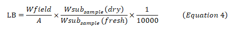
Where:
LB = Litter (biomass of litter t ha-1)
Wfield = Weight of wet field sample of litter sampled within an area of size 1 m2 (g);
A = Size of the area in which litter were collected (ha);
Wsub-sample,dry = Weight of the oven-dry sub-sample of litter taken to the laboratory to determine moisture content (g), and
Wsub-sample,fresh = Weight of the fresh sub-sample of litter taken to the laboratory to determine moisture content (g).
The percentage of organic carbon storage from the dry ash in the litter carbon pool was calculated as follows:
%Ash = (Wc - Wa) / (Wb - Wa) × 100 (5)
%C = (100 - %Ash) × 0.58 (6)
This is by considering 58% carbons in ash-free soil material.
Where:
C = Organic carbon (%),
Wa = The weight of the crucible (g),
Wb = The weight of oven dried grind samples and crucibles (g),
Wc = The weight of ash and crucibles (g).
Finally, carbon in litter t/ha for each sample was determined.
CL = LB × %C (7)
Where CL is total carbon stocks in the dead litter in t ha-1, %C is carbon fraction determined in the laboratory.
Estimation of soil organic carbon
The carbon stock density of soil organic carbon was calculated as recommended by Pearson, et al. from the volume and bulk density of the soil.
V = h × πr2 (8)
Where V is volume of the soil in the soil augur in cm3, h is the height of core sampler augur in cm, and r is the radius of augur in cm. Moreover the bulk density of a soil sample can be calculated as follows:
BD = (Wav,dry) / V (9)
Where BD is bulk density of the soil sample per, Wav,dry is average air-dry weight of soil sample per the quadrant, V is volume of the soil sample in the core sampler auger in cm3.
SOC = BD × d × %C (10)
Where:
SOC = Soil organic carbon stock per unit area (t ha-1),
BD = Soil bulk density (g cm-3),
d = The total depth at which the sample was taken (30 cm), and
%C = Carbon concentration (%)
Total Carbon Stock Density (TCSD)
The total carbon stock density of each site was calculated by adding the carbon stock densities of the individual carbon pools using the formula. In addition, it is recommended that any individual carbon pool of the given formula can be ignored if it does not contribute significantly to the total carbon stock [13].
Carbon stock density of a study area:
Cdensity = CAGB + CBGB + CLit + SOC (11)
Where:
Cdensity = Carbon stock density for all pools (t ha-1)
CAGB = Carbon in above-ground tree biomass (t C ha-1)
CBGB = Carbon in below-ground biomass (t C ha-1)
CLit = Carbon in dead litter (t C ha-1)
SOC = Soil organic carbon
The total carbon stocks were then converted to tons of CO2 equivalent by multiplying it by 44/12, or 3.67.
Scaling up AGB via remote sensing
Remote sensing facilitates the scaling-up of the plot-level AGB measurements by fine-resolution mapping to a broad spatial extent. Satellite data was used to estimate the Yeraba state forest carbon stock potential. Remote sensing based information has become an essential tool for global monitoring of natural and anthropogenic patterns, processes, and trends in continuous and repeatable observations over large areas. There are so many satellites that can predict biomass but, the cost and access of the imagery restricted the usage and selection of imageries. Recently launched free Sentinel imagery offers a better opportunity than other freely accessed satellite imageries for forest AGB mapping and monitoring which in turn helps to estimate the carbon storage [14].
Using the ESA Sen2Cor 2.80 processor built into the sentinel-2 satellite, the downloaded level-1 Top-of-Atmosphere (TOA) data were atmospherically adjusted, radiometrically calibrated, and converted to reflectance to produce level-2 Bottom-of-Atmosphere (BOA) outputs. Using the ESA Sen2Cor 2.80 processor found in the Sentinels Application Platform (SNAP) 7.0 software, the downloaded sentinel-2 level-1 Top of Atmosphere (TOA) data were atmospherically corrected, radiometrically calibrated, and converted to reflectance to produce Bottom of Atmosphere (BOA) level 2A products. The Sentinel-2 bands (2, 3 and 8) that were initially recorded at 10 m resolution were resampled to 20 m using the closest neighbor method in order to match the resolution of the SWIR band. Sentinel-2 images were mosaicked and then cropped to fit the study area's perimeter. Five vegetation indicators were created using sentinel-2 reflectance data in this study and compared to measurements of aboveground biomass taken on the ground to estimate AGC of the chosen sites. The information about vegetation indices chosen from the literature based on their ability to produce findings for aboveground biomass in the field that had greater coefficients of determination (R2) and higher correlation (r) values is shown in the Table 3 below [15].
| No | Vegetation indices | Formula |
|---|---|---|
| 1 | NDII/Normalized difference VI) | (B8-B12)/(B8+B12) |
| 2 | ARVI /Atmospheric resistant VI) | (B8-(B4-B2))/(B8+(B4) |
| 3 | GNDVI /Green normalized difference VI) | (B8-B3)/(B8+B3) |
| 4 | VDVI (Visible band difference VI) | (2*green-red-blue)/(2*green + red + blue) |
| 5 | NDVI (Normalized difference VI) | (B8-B4)/(B8+B4) |
Table 3: General information of sentinel 2A MSI level 1c spectral Vegetation Indices (VI).
Correlation and regression statistical data analysis
Field above ground biomass and carbon stock analysis was done using excel. Vegetation indices from sentinel 2 satellite images were calculated under ArcGIS 10.8 software using raster calculator. Field plots laid on the vegetation index values using the sample plots latitude and longitude. Since forest AGB data were recorded in 20 m × 20 m grid, mean values of Vegetation indices of each sample plot extracted using 20 m × 20 m rectangular grid in ArcGIS 10.8 as shown in Figure 6 below.

Figure 6: Workflow.
Producing carbon sink and stock potential map of the forest
After the above and Below Ground SOC content of the individual plots in Yeraba state forest determined; the total carbon sink potential of the individual plots was also added to quantify the above and below carbon content. In addition, in order to produce the total carbon sink potential map of the forest, GCPs of the individual sample plots collected using GPS. Thus, the quantified total carbon sequestration potential and the GCPs of the individual ample plots were tabulated together and added into Arc map compatible data. After that the corresponding GCPs and quantified carbon sequestration potential of the whole sample plots were overlaid on the Arc map Graphic Interface by points. Finally the Inversed Distance Weight (IDW) method of interpolation was used for estimation of spatial distribution of biomass by Arc map 10.8. The reason that choosing IDW interpolation is that the method provides accurate biomass estimation than kriging for estimating spatial distribution of biomass [16].
Results
Field above ground biomass of the study area
Following the collection of field data, the study area's above-ground biomass and carbon stock were calculated using an allometric equation created by earlier researchers. The allometric formula that calculates the AGB based on the tree's needed height, its Diameter at Breast Height (DBH), and the species' individual wood densities. The field data was translated into above-ground biomass (t/ha) and above-ground carbon (t/ha) for each plot using the values as true biomass and carbon values for each plot. Based on biomass, the carbon content of each sample plot was estimated by adding the biomass produced by each species that was present there (Figures 7 and 8).
Utilizing the allometric derivation of the wood density of various species, height, and DBH data gathered from 17 sample plots, the above-ground biomass is calculated. As per the IPCC recommendation, 909 trees totaling greater than or equal to 5 cm DBH were counted in this study region and measured in the field to estimate the above-ground tree biomass and carbon. Field data's AGB value ranges from 73.79973 tons per plot to 2.19183 tons per plot. The greatest and minimum AGB are found in the second and eighth sample plots, respectively, out of all the plots. In contrast to the other six plots, which are sparse, long, and thickly vegetated, the seventh plot is dense, thin, short, and youthful (Table 4) [17].
| N | Min | Max | Rang | Median | Mean | Sum | |
|---|---|---|---|---|---|---|---|
| AGB/ton | 17 | 2.19183 | 73.79973 | 71.6079 | 9.509017 | 18.03275 | 306.5567 |
Table 4: Shows field above ground biomass of the study area.

Figure 7: DBH and Tree height class distribution.

Figure 8: AGB distribution per plot.
Comparison of vegetation indices for AGB/AGC estimation
The researcher created equations for the calculation of aboveground carbon stock using data from the relationship analysis of the field survey data and sentinel 2 data. The Above-Ground Carbon Stock (AGCS) value and the Vegetation Index value obtained from sentinel 2 were compared in this study using Pearson's correlation. It assesses how strongly two variables are linearly related. A close correlation between them can be inferred if the coefficient was near to 1. On the basis of an identifying tool, the pixel values for each sample were retrieved. These samples' image values were retrieved, and the correlation's strength, pattern, and equation were then examined. Model of each parameter are explained by using the regression correlation analysis. Regression models that are as linear as possible are utilized in the investigation to determine the correlation pattern. When vegetation canopies are not homogeneous in terms of species, which causes complexity and variance in groundcover, evaluating many vegetation indices is important. Since various ranges of biomass and groundcover have distinct indices that are more sensitive, factors like terrain, background soil reflectance, and variance in internal canopy signal scattering may affect the final vegetation signal. Based on this, the sentinel 2A MSI level 1C sensor's 20/02/2023 reading of 5 (five) vegetation indices was derived as Figure 9 depict [18].

Figure 9: VI’s map of the study area.
Correlation of AGB/AGC with VDVI
The correlation between AGCS values and VDVI as illustrated in Figure 10, the coefficient of correlation was approximately 0.65 which showed that VDVI has performed high as compared to other indices (NDII, NDVI, GNDVI, and ARVI). Therefore VDVI was the best vegetation index that corresponded to AGCS the regression model of VDVI can explain 65% of field data while 35% of the data variations remain unexplained. In general, the result indicates that there is a strong positive correlation linear relationship between VDVI and above ground carbon stock. This shows that the VDVI average is a good indicator of the above-ground carbon stock estimation than the remaining one [19].

Figure 10: AGB and VDVI relationship.
Correlation of AGB/AGC with NDVI
The correlation between AGCS values and Vegetation Index (NDVI) values computed from sentinel 2 image has been shown in Figure 11. As represented in the scatter plot; the coefficient of correlation was 0.5974 which showed that NDVI model was capable to explain 59.74% of field data while the remaining 40.26% of the data are not explained by this model. The NDVI model has performed well than others except VDVI [20].

Figure 11: Correlation of AGB/AGC with NDVI.
Correlation of AGB/AGC with ARVI
The correlation between AGCS values and Vegetation Index (ARVI) values computed from Sentinel 2 image has been shown in Figure 12. As represented in the scatterplot; the coefficient of correlation was 0.5801 which showed that ARVI model was capable to explain 58.01% of field data while the remaining 40.26% of the data are not explained by this model. The ARVI model has not performed well when it compared with the two above models [21].

Figure 12: Correlation of AGB/AGC with ARVI.
Correlation of AGB/AGC with NDII
The correlation between AGCS values from field data and NDII values derived from sentinel 2 image has been shown in Figure 13. As represented in the scatterplot, the coefficient of correlation was 0.534 which showed that the relationship between NDII and AGCS is not too much strong as compared to the rest of the indices (VDVI, NDVI, and ARVI), but it performs well as compared to GNDVI. The regression NDII model can explain only 53.4% of the variation in AGCS data while 56.6 % of the data is not explained by this model.

Figure 13: Correlation of AGB/AGC with NDII.
Correlation of AGB/AGC with GNDVI
GNDVI derived from sentinel 2 was computed for correlation with above-ground carbon stock. As a result Figure 14 shows the scatter plot of carbon stock versus GNDVI weak when it compared with the above remaining vegetation indices.

Figure 14: Correlation of AGB/AGC with GNDVI.
Modeling the relationship between AGC and VIs
Linear regression models were developed based on the integration of AGCS data and vegetation indices derived from sentinel 2. The result provides a comparison of the best regression models identified according to a multiple vegetation index. The R-value of vegetation indices ranges from 0.76 to 0.81, and R2 varied between 0.51 and 0.65. All vegetation indices showed a significant and positive correlation with AGCS. VDVI was the best vegetation index that corresponded to AGCS (r=0.81 and R2=0.65) followed by NDVI, ARVI, NDII, and GNDVI (Tables 5-8) [22].
| No | VI’s | R | R2 | significance |
|---|---|---|---|---|
| 1 | ARVI | 0.76 | 0.58 | 0 |
| 2 | GNDVI | 0.71 | 0.51 | 0 |
| 3 | VDVI | 0.81 | 0.65 | 0 |
| 4 | NDII | 0.73 | 0.53 | 0 |
| 5 | NDVI | 0.77 | 0.6 | 0 |
Table 5: Statistical result of the relationship between AGC and Vis.
| Summary output | |
|---|---|
| Regression statistics | |
| Multiple R | 0.81 |
| R square | 0.65 |
| Adjusted R square | 0.63 |
| Standard error | 12.68 |
| Observations | 17 |
Table 6: Summary output of regression statistics.
| ANOVA | |||||
|---|---|---|---|---|---|
| df | SS | MS | F | Significance F | |
| Regression | 1 | 4465.56 | 4465.55 | 27.75 | 0 |
| Residual | 15 | 2413.53 | 160.9 | ||
| Total | 16 | 6879.08 |
Table 7: ANOVA.
| Coefficients | Standard error | t Stat | P-value | Lower 95% | Upper 95% | Lower 95.0% | Upper 95.0% | |
|---|---|---|---|---|---|---|---|---|
| Intercept | 3.26 | 4.16 | 0.78 | 0.45 | -5.62 | 12.13 | -5.62 | 12.13 |
| VDVI | 57.24 | 89.08 | 5.27 | 0 | 279.43 | 659.18 | 279.43 | 659.18 |
Table 8: Intercept.
Log (AGB) = (VDVI × 57.24) + 3.26 (12)
Log (AGC) = (VDVI × 57.24) + 3.26 + 0.47 (13)
Correlation of field AGB and predicted AGB
Predicted above ground biomass extracted from pixels at the samples location was correlated with the observed above ground biomass to decide the effectiveness of the model to predict AGB for other pixels. According to Figure 15, the coefficient of determination (R2=0.6) and correlation coefficient (r=0.77) shows strong relationship between the observed and predicted AGB. As a result the model generated through linear regression was used to map the final map of AGB for the study area.

Figure 15: Correlation of field AGB and predicted AGB.
Above-ground carbon stock distribution map
According to Houghton, forest has large potential for temporary and long term storage of carbon. As the study showed that, different tree species had different carbon stock potential. A large amount of carbon stock has been observed in a species which has counted long lived in the study site and also species which are densely populated in the study area. As a result this study indicates unbalanced tendency of carbon stock input in the above ground of the site. Among 6 major tree species in the study site high biomass rate has been recorded by species such as Cupressus lusitanica, Eucalyptus globuse, Acacia dicurusne, Pinus patula, Acacia melanoxylon and Grevillea roubsta.
Species-specific allometric models were applied to field allometric measurements to produce AGC ground truth estimates for each of the 17 plots and scaling up with sentential data. Based on the model AGB was predicted for the whole study sites. Finally the AGB values were converted in to AGC results. As the Figure 16 depicts that the result of AGC Yeraba state forest lies between 5 ton/pixel to 39.72 ton/pixel. Based on the result which illustrated in the below Figure 16 about 15.32%, 22.76%, 39.12%, 21.7% and 1.1% of the study forest has an AGC from 5.005–18.349 ton, 18.349–22.842 ton, 22.842–26.654 ton, 26.654–31.566 ton and 31.566–39.725 per pixel respectively. The mean value and standard deviation of carbon being stored was 23.4 and 4.396 ton. The total carbon stored by the study forest was about 183745.52 ton. As the Figure 16 showed that above ground carbon stock varied in magnitude, the highest concentration of AGC was concentrated southern part of the forest, as the area was covered with tall and long Eucalyptus trees on the other hand central part of the study forest was accounted less concentration of AGC due to the area was covered by sparse vegetation and most part of the area was occupied by grass.

Figure 16: Above-ground carbon stock distribution map.
Below ground carbon potential
Below ground carbon is another forest carbon pool which derivate from the AGC. As a result the pattern of distribution is similar with AGC except its value dedication. Similarly, BGC also varied in terms of magnitude. The highest concentration of BGB was concentrated around northern and southern central part of the study forest on the other hand central part of the study area was less concentration of BGC. As the Figure 17 illustrated that, the result of BGC varies from 1.031 ton/pixel to 10.326 ton/pixel. The mean value, standard deviation and total carbon being stored were 6.121, 1.142 and 47637.336 ton. Based on the result which present in the below Figure 17, about 15.6%, 22.96%, 39.14%, 21.2% and 1.1% of the study forest has an AGC from 1.301–4.806 ton, 4.806–5.974 ton, 5.974–6.965 ton, 6.965–8.24 ton and 8.24–10.328 per pixel respectively.

Figure 17: Below ground carbon potential.
Litter carbon stock potential
The forest carbon is found in all living/dead erected trees, roots, herbaceous trees and litters. All the fallen leaves, grasses and fine branches found in the study were considered as litter. The collected samples of 1 m × 1 m size in five points of a plot and mixed to one sample resulting 17 litter samples were gathered and tested in laboratories. The highest and lowest carbon stock was observed in plot 7 and plot 14 with carbon stock of 4.58 ton and 2.7 ton respectively (Figures 18 and 19).

Figure 18: Litter carbon stock potential.

Figure 19: Litter carbon (distribution/plot).
Estimation of Carbon Stocks in (SOC)
Bulk density: The bulk density was computed on the soil profile. The bulk density of the study soil was 0.377 gcm-3 minimum value and 0.44 g cm-3 maximum value with a mean value of 0.408 g cm-3. Generally there is no significant difference between maximum and minimum bulk density.
Soil organic carbon: The laboratory results for the organic carbon of the sample soils are shown in (Appendix). The result showed that, the highest percentage of organic carbon was 12.63% which observed at plot 2: whereas, 8.25% is the lowest value which indicated at plot 3 and the mean percentage value of organic carbon in this pool is 9.77.
Soil carbon stock: In the study area the minimum and maximum carbon stock in the soil was 95.153 ton/plot which locate at plot 15 and 157.978 ton/plot at plot 2 with mean total carbon stock of 119.679 ton/plot (Figures 20 and 21).

Figure 20: Soil carbon stock map.

Figure 21: Soil carbon (ton).
Total carbon stock of Yeraba state forest
The total carbon stock of the study area was done by summing up all the carbon value of each pool (above ground and below ground carbon, litter carbon and soil organic carbon) for all plot samples of the study area by using weighted sum overlay technique. The carbon values of the study forest ranged from a minimum of 191.93 to a maximum of 625.79 ton/hectare. The average carbon density in all carbon pool of the study area was 408.86 ton/hectare (Figure 22).

Figure 22: Total carbon stock of Yeraba state forest.
Influences of environmental factors on carbon stock
Variation of carbon stock along altitudinal gradient:
The variety, biomass, and carbon stock in forest ecosystems are known to be significantly influenced by altitude although there is a slight differential in carbon stock with respect to the altitudinal gradient in this study region, there is no discernible altitudinal variation. The highest elevation class of the study region was where the largest AGC values were found, while the lowest elevation class was where the least AGC values were found. The mean value of the AGC decreased from the highest to the lowest elevation when we compared the mean values in terms of altitudinal variance. The same is true of BGC, which is an ancestor of AGC. Because a few large individuals can account for a significant amount of the quadrats above and below ground carbon, the presence of species with large individuals at high altitudes may have an impact on AGB and carbon stock.
The mean carbon density in litter pool and soil pool of the present study was not showed clear pattern with altitude, but they had showed relatively an increasing trend with increasing altitude though there was no significant variation due to the elevated area of the study part was characterized by sparse, tall, and thick trees and their leaves can fall down easily towards the ground. The detail values were presented below table (Figure 23 and Table 9).
| Elevation class | Min. | Max. | Range | Mean | Std. | Sum |
|---|---|---|---|---|---|---|
| AGC | ||||||
| 2395-2427 m | 6.71 | 34.64 | 27.93 | 21.88 | 3.75 | 38930.67 |
| 2427-2460 m | 11.06 | 32.96 | 21.9 | 23.22 | 4.17 | 99346.66 |
| 2460-2493 m | 13.72 | 39.73 | 26 | 26.65 | 3.95 | 44671.82 |
| BGC | ||||||
| 2395-2427 m | 1.75 | 9.01 | 7.26 | 5.69 | 0.97 | 10121.97 |
| 2427-2460 m | 2.88 | 8.57 | 5.69 | 6.04 | 1.09 | 25830.13 |
| 2460-2493 m | 3.57 | 10.33 | 6.76 | 6.93 | 1.03 | 11614.67 |
| LC | ||||||
| 2395-2427 m | 2.75 | 4.3 | 1.55 | 3.38 | 0.34 | 6018.19 |
| 2427-2460 m | 2.43 | 4.52 | 2.09 | 3.38 | 0.45 | 14471.04 |
| 2460-2493 m | 2.54 | 4.58 | 2.04 | 3.57 | 0.47 | 5985.56 |
| SOC | ||||||
| 2395-2427 m | 95.23 | 151.58 | 56.35 | 119.27 | 11.26 | 212057.6 |
| 2427-2460 m | 104.15 | 157.98 | 53.83 | 120.28 | 8.03 | 514557.5 |
| 2460-2493 m | 99.21 | 153.78 | 54.57 | 121.38 | 10.66 | 203429.4 |
| TC | ||||||
| 2395-2427 m | 213.78 | 574.4 | 360.62 | 398.42 | 50.1 | 708385.3 |
| 2427-2460 m | 262.04 | 540.99 | 278.94 | 416.19 | 53.11 | 1780063 |
| 2460-2493 m | 296.73 | 625.79 | 329.06 | 460.79 | 47.75 | 772279.9 |
Table 9: Each carbon pool statistical values with elevation class/ton.

Figure 23: Elevation class of the study area.
Distribution of carbon stock along slope gradient:
Slope is also one of the environmental factors that influence the distribution of carbon density. As indicated in, the carbon partitioning among forest carbon pools along slope gradients is important in knowing possible change in carbon stock and thus carbon stock potential in response to the future climate change in mountain regions. The maximum above ground carbon was recorded at the lowest slope class (0–10%) followed by middle class (10–20%) and the higher class (20–31%). On the other hand, minimum AGC was located at the middle class of slope (10–20%), followed by lowest slope class (0–10%) and higher class (20–31%) and its mean AGC carbon stock value is similar pattern as indicated in the following table. The same is true for BGC stock of the study area.
Litter carbon and soil carbon stock also insignificant variation along slope inclination, but the minimum and maximum carbon stock for litter carbon pool was found in middle class followed by lower and upper class. On the other hand, the maximum carbon stock for this pool also recorded at middle class followed by upper and lower class. The values of SC in this study area also have slit greater the lower part of the study area as the transported soil accumulated in flat surface. The maximum TC was recorded at the middle class next at lower and upper class (Figure 24 and Table 10).
| Slope class | Count | Min. | Max. | Range | Mean | Std. | Sum |
|---|---|---|---|---|---|---|---|
| AGC | |||||||
| 0-10% | 4323 | 12.23 | 39.73 | 27.5 | 23.61 | 4.44 | 102052.9 |
| 10-20% | 2929 | 11.72 | 35.73 | 24.01 | 24.1 | 4.16 | 70591.83 |
| 20-31% | 164 | 12.45 | 30.72 | 18.26 | 23.46 | 4.26 | 3847.12 |
| BGC | |||||||
| 0-10% | 4323 | 3.18 | 10.33 | 7.15 | 6.14 | 1.15 | 26533.75 |
| 10-20% | 2929 | 3.05 | 9.29 | 6.24 | 6.27 | 1.08 | 18353.88 |
| 20-31% | 164 | 3.24 | 7.99 | 4.75 | 6.1 | 1.11 | 1000.25 |
| LC | |||||||
| 0-10% | 4323 | 2.45 | 4.54 | 2.09 | 3.36 | 0.46 | 14535.31 |
| 10-20% | 2929 | 2.43 | 4.58 | 2.15 | 3.51 | 0.41 | 10272.43 |
| 20-31% | 164 | 2.85 | 4.56 | 1.71 | 3.68 | 0.39 | 603.47 |
| SOC | |||||||
| 0-10% | 4323 | 95.23 | 157.98 | 62.75 | 120.75 | 9.32 | 522010.5 |
| 10-20% | 2929 | 96.48 | 156.41 | 59.92 | 119.87 | 9.61 | 351086.7 |
| 20-31% | 164 | 97.95 | 151.78 | 53.83 | 120.1 | 11.95 | 19695.93 |
| TC | |||||||
| 0-10% | 4323 | 274.51 | 625.79 | 351.28 | 421.56 | 57.11 | 1822412 |
| 10-20% | 2929 | 277.16 | 575.52 | 298.36 | 427.05 | 52.57 | 1250816 |
| 20-31% | 164 | 279.69 | 505.76 | 226.07 | 419.35 | 55.25 | 68773.12 |
Table 10: Each carbon pool statistical values along slope gradient.

Figure 24: Slope class of the study area.
Distribution of carbon stock in the aspects (slope facings):
Aspect is one of environmental factors that can affect the carbon stock of forests in different carbon pools and thus, it can be used as a useful variable to forecast the forest carbon stock in different carbon pools (Figure 25). Aspect has significant relationship with bio-mass carbon in forest areas due to the interaction between solar radiation and soil properties. As below Table 11 depict that the maximum values of AGC and BGC were recorded towards northeastern aspect part of the study whereas the lowest values of the above carbon pool values were located towards western part of the study site. This may be related to the timing of sunlight that the vegetation can absorb. That means the vegetation that have been grown in the East direction receive sunlight earlier than vegetation in West and other directions.

Figure 25: Aspect Class of the Study Area.
| Aspect class | Count | Min | Max | Range | Mean | Std | Sum |
|---|---|---|---|---|---|---|---|
| AGC | |||||||
| North (0-22.5) | 941 | 13.09 | 39.3 | 26.21 | 24.22 | 4.01 | 22789.92 |
| Northeast (22.5-67.5) | 347 | 13.77 | 39.73 | 25.95 | 23.29 | 4.39 | 8081.37 |
| East (67.5-112.5) | 652 | 12.81 | 39.42 | 26.61 | 23.96 | 4.34 | 15621.87 |
| Southeast (112.5-157.5) | 1049 | 13.65 | 38.9 | 25.25 | 23.97 | 4.33 | 25148.79 |
| South (157.5-202.5) | 1106 | 12.86 | 38.55 | 25.69 | 24 | 4.25 | 26548.4 |
| Southwest (202.5-247.5) | 781 | 13.07 | 38.18 | 25.11 | 23.68 | 4.3 | 18492.21 |
| West (247.5-292.5) | 651 | 12.23 | 39.22 | 26.99 | 23.88 | 4.64 | 15543.93 |
| Northwest (292.5-337.5) | 1105 | 12.68 | 39.11 | 26.43 | 23.76 | 4.32 | 26253.56 |
| North (337.5-360) | 423 | 12.42 | 39.52 | 27.1 | 23.81 | 4.75 | 10073.71 |
| BGC | |||||||
| North (0-22.5) | 941 | 3.4 | 10.22 | 6.82 | 6.3 | 1.04 | 5925.38 |
| Northeast (22.5-67.5) | 347 | 3.58 | 10.33 | 6.75 | 6.06 | 1.14 | 2101.16 |
| East (67.5-112.5) | 652 | 3.33 | 10.25 | 6.92 | 6.23 | 1.13 | 4061.69 |
| Southeast (112.5-157.5) | 1049 | 3.55 | 10.12 | 6.57 | 6.23 | 1.13 | 6538.68 |
| South (157.5-202.5) | 1106 | 3.34 | 10.02 | 6.68 | 6.24 | 1.1 | 6902.58 |
| Southwest (202.5-247.5) | 781 | 3.4 | 9.93 | 6.53 | 6.16 | 1.12 | 4807.97 |
| West (247.5-292.5) | 651 | 3.18 | 10.2 | 7.02 | 6.21 | 1.21 | 4041.42 |
| Northwest (292.5-337.5) | 1105 | 3.3 | 10.17 | 6.87 | 6.18 | 1.12 | 6825.92 |
| North (337.5-360) | 423 | 3.23 | 10.28 | 7.05 | 6.19 | 1.23 | 2619.16 |
| LC | |||||||
| North (0-22.5) | 941 | 2.47 | 4.58 | 2.11 | 3.39 | 0.47 | 3187.11 |
| Northeast (22.5-67.5) | 347 | 2.48 | 4.53 | 2.04 | 3.39 | 0.44 | 1177.74 |
| East (67.5-112.5) | 652 | 2.53 | 4.47 | 1.93 | 3.42 | 0.45 | 2232.4 |
| Southeast (112.5-157.5) | 1049 | 2.45 | 4.47 | 2.03 | 3.39 | 0.44 | 3560.57 |
| South (157.5-202.5) | 1106 | 2.45 | 4.51 | 2.06 | 3.44 | 0.43 | 3804.26 |
| Southwest (202.5-247.5) | 781 | 2.43 | 4.54 | 2.11 | 3.43 | 0.46 | 2680.44 |
| West (247.5-292.5) | 651 | 2.44 | 4.57 | 2.13 | 3.42 | 0.46 | 2228.05 |
| Northwest (292.5-337.5) | 1105 | 2.45 | 4.57 | 2.13 | 3.49 | 0.44 | 3861.01 |
| North (337.5-360) | 423 | 2.47 | 4.55 | 2.08 | 3.45 | 0.45 | 1459.89 |
| SC | |||||||
| North (0-22.5) | 941 | 95.65 | 157.6 | 61.95 | 120.78 | 10 | 113650.5 |
| Northeast (22.5-67.5) | 347 | 99.27 | 154.69 | 55.42 | 119.8 | 9.49 | 41571.57 |
| East (67.5-112.5) | 652 | 99.98 | 156.23 | 56.24 | 120.06 | 8.28 | 78281.59 |
| Southeast (112.5-157.5) | 1049 | 97.76 | 157.23 | 59.47 | 121.39 | 9.64 | 127342.4 |
| South (157.5-202.5) | 1106 | 97.68 | 157.55 | 59.86 | 120.96 | 9.9 | 133785.8 |
| Southwest (202.5-247.5) | 781 | 95.25 | 157.98 | 62.72 | 119.45 | 8.94 | 93288.99 |
| West (247.5-292.5) | 651 | 96 | 157.13 | 61.12 | 119.68 | 8.72 | 77913.6 |
| Northwest (292.5-337.5) | 1105 | 95.27 | 157.63 | 62.36 | 121 | 10.1 | 133699.8 |
| North (337.5-360) | 423 | 100.16 | 153.04 | 52.88 | 119.51 | 8.84 | 50552.12 |
| TC | |||||||
| North (0-22.5) | 941 | 287.72 | 620.17 | 332.45 | 429.32 | 51.38 | 403990.6 |
| Northeast (22.5-67.5) | 347 | 296 | 625.79 | 329.79 | 416.64 | 55.46 | 144574.6 |
| East (67.5-112.5) | 652 | 284.38 | 621.83 | 337.45 | 425.38 | 55.47 | 277349.6 |
| Southeast (112.5-157.5) | 1049 | 293.28 | 614.81 | 321.54 | 426.86 | 55.65 | 447777.7 |
| South (157.5-202.5) | 1106 | 283.16 | 609.98 | 326.82 | 426.85 | 54.35 | 472100 |
| Southwest (202.5-247.5) | 781 | 284.67 | 605.63 | 320.96 | 421.22 | 54.91 | 328971.2 |
| West (247.5-292.5) | 651 | 274.51 | 619.17 | 344.67 | 423.96 | 59.1 | 275995.2 |
| Northwest (292.5-337.5) | 1105 | 278.94 | 618.39 | 339.45 | 423.85 | 55.47 | 468355.6 |
| North (337.5-360) | 423 | 279.66 | 623.7 | 344.03 | 423.03 | 60.25 | 178940.8 |
Table 11: Each carbon pool statistical values along aspect variation.
Discussion
Woody species composition
Yeraba state Forest is characterized by major dominant species like, Acacia decurrens, Eucalyptus globulus, Acacia melanoxylon, Grevillea roubsta and Pinus patula and it had different species composition, DBH, height, density and frequency. In addition, the area was characterized by insignificant altitudinal range that lies (2395–2493 m) and its slope inclination found between 0 and 31%.
Woody species composition of the given vegetation can be described in terms of its richness in species, abundance, dominance, and frequency. As the study forest is state forest (planted by human intervention) the area was characterized by a few but high frequency distribution of six wood species. The study forest was covered with a great proportion of Cupressus lusitanica (52.63%) followed by Eucalyptus globuse (16.89%), Acacia dicurusne (10.39%), Pinus patula (8.22%), Acacia melanoxylon (7.42%) and Grevillea roubsta (4.45%). According to Lambrecht (1989), frequency is the indication of homogeneity and heterogeneity of vegetation. High value in higher frequency and low value in lower frequency classes reveal constant or similar composition. On the other hand, high percentage of number of species in the lower frequency classes and low percentage of number of species in the higher frequency classes indicates a high degree of floristic heterogeneity. The species that appear in lower frequency classes have irregular occurrence whereas those appearing in higher classes have regular horizontal classes. The present study revealed that there is high percentage number of species in higher frequency classes and low percentage number of species in lower frequency classes. This indicates that the forest under the study has high degree of floristic homogeneity and low heterogeneity.
DBH and height arrangement of trees and their contribution in the studied forest
Tree species with the highest average DBH in the study forest were like Eucalyptus globuse (28.22 cm) followed by Acacia melanoxylon (22.56 cm), Cupressus lusitanica (14.32 cm), Acacia dicurusne (9.12 cm), Pinus patula (8.89 cm), and Grevillea roubsta (8.79 cm). The reason why Pinus patula and Grevillea roubsta were minimum average DBH is that all are young as they were planted recent. The remaining were planted at the beginning where the study forest was emerged.
Tree species with highest average height in the study forest were Acacia melanoxylon (16.41 m) followed by Eucalyptus globuse (15.74 m), Pinus patula (14.67 m), Cupressus lusitanica (10.74 m), Acacia dicurusne (7.72 m) and Grevillea roubsta (5.75 m)
Correlation of AGC with derived sentinel vegetation indices
The sentinel-2A product has comparatively large spatial coverage and high resolution to perform efficiently for estimation of biomass than other open source sensors data products. The vegetation indices derived from remote sensing data are considered to be the most sensitive to the photosynthetic parts of the plant and are related to the aboveground live biomass and growing stock. That reason of saturation is the computation of indices through NIR and Red spectral band and the red band absorb electromagnetic radiation and remain constant while the canopy cover increases hence in result at 100% canopy cover red energy absorption reaches to peak. Also, the soil reflectance and topography have impact on biomass estimation using spectral indices. Therefore, assessment of varieties of spectral indices is very useful.
In this study spearman rho correlation was tasted with five spectral indices and results showed high coefficient of correlation between the obtained characteristics of the field measurements and spectral indices. 0.71 was the lowest correlation coefficient value obtained from the correlation of GNDVI and field AGB. The highest and most robust correlation coefficient was observed between VDVI and field AGB data was 0.81. This is differ from the data obtained by and Ali, et al. who conducted large-scale studies on forest biomass in different types of forest in Europe and with who studied the correlation of vegetation indices with above ground biomass.
Regression results of the five indices were compared to see their performance in predicting above ground biomass. The results revealed that the coefficients of determination of VDVI (R2 = 0.65) followed by NDVI (R2 = 0.59), ARVI (R2 = 0.58), NDII (R2 = 0.53), GNDVI (R2 = 0.50). VDVI with coefficient of determination of 0.65 was selected from the five indices as its coefficient of determination is significant than others to analyses AGB.
Carbon stock in different pools
According to Houghton, forest has large potential for temporary and long term storage of carbon. As the study showed that, different tree species had different carbon stock potential. A large amount of carbon stock has been observed in a species which has counted long lived in the study site and also species which are densely populated in the study site. As a result this study indicates unbalanced tendency of carbon stock input in the above ground of the site.
While comparing with other studies, the mean carbon stock in above and belowground biomass of the study forest was lower than Arba Minch Water Forest 414.7 ton/hectare, Tara Gedam Forest 306.36 ton/hectare, Egdu Forest 278.08 ton/hectare and Danaba Community forest 277.78 ton/hectare but greater than Biheretsige and Central Closed Public Park 25.4 ton/hectare, Bangladesh forest 96.13 ton/hectare, Selected Church Forest 122.85 ton/hectare, Gendo Forest 128.6 ton/hectare and Menagesha Suba State Forest 133 ton/hectare. Generally, the mean above ground carbon values recorded in the study sites were above two fold the values recommended by IPCC for tropical dry forest 65.00 t/ha. According to different literature, global above ground carbon in tropical dry and wet forests ranged between 13.5–122.85 t/ha and 95–527.85 t/ha, respectively. As BGC was obtained from AGC its increment and decrement is similar with AGC.
The amount of litter fall and its carbon stock of the forest can be influenced by the forest vegetation (species, age and density) and climate. Similarly, the tree stands in the forest area were relatively still young and this could result in low amount of litter fall. In addition, since the study area is located in tropical areas, the rate of decomposition is relatively fast. Thus, the lowest carbon stock in litter pool could probably be due to the high decomposition rate and less amount of litter fall. As Table 12 below illustrated that like AGC and BGC the values of LC and SOC also vary from other studies.
According to Brown and Lugo litter fall in dry tropical Forests range between 2.52–3.69 t/ha. The dead litter carbon stock estimated in Addis Ababa church forests ranged from 3.37 to 7 t/ha. Carbon stock of metti mountain forest-wechecha, West Oromia, Ethiopia ranged from 6.1–15.7 tons. Dead litter carbon in the present study range from 2.53–4.58. Forest which is higher than the values reported for dry tropical Forests whereas less than the remaining which is listed above. The amount of litter fall and its carbon stock of the forest can be influenced by the forest vegetation (species, age and density) and climate.
Comparison different studies with current study
Different studies were conducted on the carbon stock estimation of Forests in different parts of Ethiopia. The results of all studies were varying from place to place and time to time due to different reasons as show below Table 12.
| Study place | AGC | BGC | LC | SC |
|---|---|---|---|---|
| Selected church forest | 122.85 | 25.97 | 4.95 | 135.94 |
| Menagesha suba state forest | 133 | 26.99 | 5.26 | 121.28 |
| Egdu forest | 278.08 | 55.62 | 3.47 | 277.56 |
| Tara gedam forest | 306.36 | 61.52 | 0.9 | 274.32 |
| Arba minch water forest | 414.7 | 83.48 | 1.28 | 83.8 |
| Bangladesh forest | 96.13 | 14.6 | 4.2 | 168.15 |
| Danaba community forest | 277.78 | 41.65 | 1.06 | 186.4 |
| Humbo forest | 107.927 | 50.72 | 17.85 | 185.13 |
| Biheretsige and central closed public park | 25.4 | 5.1 | 5.17 | 113.55 |
| Gendo forest | 128.6 | 26.52 | 3.12 | 94.96 |
| Present study | 223.656 | 58.15 | 3.41 | 119.679 |
Table 12: Comparison different studies with current study.
Conclusion
From this study, it has been found that the study forest has limited woody Plant species with diversified vegetation character like DBH, tree height, density and the like. The researcher designed measurable objectives by stating objectives: To estimate carbon stock in above, below, litter and soils, Assess the correlation of AGB/AGC with sentinel 2A derived vegetation indices, produce carbon stock potential map for the study area, to illustrate the distribution of carbon stock with surface data. The heterogeneous carbon stock in this forest area can be attributed to the difference in specific wood density, tree height, DBH as well as in other biotic and abiotic factors affecting the tree growth. Average carbon stocks of the different carbon pools of this study were comparatively similar with most researches done in Ethiopia in carbon stock potentials of forests.
Altitudinal gradient has insignificant impact over forests above ground biomass as well as tree species diversity as the area is characterized insignificant altitudinal variation. Even the study forest has a little elevation range, the highest elevation class of the study region was contain the largest AGC values were found, while the lowest elevation class was stored the least AGC values were found. The mean carbon density in the soil and litter pool of the current study did not show a clear pattern with altitude. Slope and slope aspect also influence the distribution of carbon stock potential of the study area.
Recommendations
The integration of remote sensing and ground based data to estimate carbon stock potential of the study area provide plausible output in this study. But for further improvement on the following points are recommended by the researcher.
Estimating forest carbon stocks using optical images may be subject to the saturation problem because of the density of the forest. Furthermore, the canopy penetration capabilities of sentinel2A and Landsat 5 images are inadequate. The effectiveness of carbon stock estimation for future studies may be improved by the use of LiDAR and Radar imageries that can tackle the saturation and canopy penetration problems.
Research findings, such as socioeconomic, ethno botanical, and in-depth ecological studies in relation to various environmental aspects, such as soil type and characteristics, should aid in the development and management of the Forest. In contrast, basic and applied research into the soil seed bank, seed physiology, population dynamics, the biology and ecology of endangered species, as well as the forest as a whole, should be done to fill the gaps in this effort.
Acknowledgements
First and for most I would like to thank the almighty God for being with me all the time, who makes everything possible and giving me everything to accomplish my work. I am very grateful to my advisors, Dr. Mesfin Anteneh for his constructive criticisms, comments, and unreserved efforts as needed in running this study.
I am also thankful to Bahir Dar University all Geography and Environmental studies staff members for their friend hood approach, suggestions, moral and material support. Generally, who supported me directly or indirectly for the accomplishment of this MSc thesis, thank you so much!
I would like to express my deepest thankful and gratitude for my beloved wife Yenguse Desibel for her unlimited support with moral and make me strong to accomplish this thesis and gives me road map of passing obstacles from beginning to the finish.
I am also indebted for my friends Andargie Abebayehu (camera man and photo editor) and Yeshwas Mengistu (whole seller) who supported and encouraged me morally and ideally throughout my work.
I am also thankful to Baso liben woreda public library staff who facilitation the library to completing this study. Additionally I have also a great gratitude for Baso liben woreda Land office and agricultural office staffs especially for Mr. Abebaw Yitayeh who support with moral and materials to collect the valuable data for this study.
Lastly, I would like to appreciate all with me in all aspect was not listed in this paper.
References
- Allan J, Mitchell T, Harborne N, Bohm L, Crane-Robinson C. Roles of H1 domains in determining higher order chromatin structure and H1 location. J Mol Biol. 1986;187(4):591-601.
[Crossref ] [Google Scholar] [PubMed]
- Alves LF, Vieira SA, Scaranello MA, Camargo PB, Santos FA, Joly CA, et al. Forest structure and live aboveground biomass variation along an elevational gradient of tropical Atlantic moist forest (Brazil). For Ecol Management. 2010;260(5):679-691.
[Crossref] [Google Scholar] [PubMed]
- Eshetu AA. Forest resource management systems in Ethiopia: Historical perspective. IJBC. 2014;6(2):121-131.
- Anderson-Teixeira KJ, Herrmann V, Morgan RB, Bond-Lamberty B, Cook-Patton SC, Ferson AE, et al. Carbon cycling in mature and regrowth forests globally. Environ Res Lett. 2021;16(5):053009.
- Andrew RM. Global CO2 emissions from cement production, 1928–2018. Earth Syst Sci Data. 2019;11(4):1675-1710.
- Effiom AE. UAV-RGB and Multispectral Pleiades images, for tree species identification and forest carbon estimation in Amtsvenn, Germany (Master's thesis, University of Twente).
- Ayanu YZ, Conrad C, Nauss T, Wegmann M, Koellner T. Quantifying and mapping ecosystem services supplies and demands: a review of remote sensing applications. Environ Sci Technol. 2012;46(16):8529-8541.
[Crossref] [Google Scholar] [PubMed]
- Bekele-Tesemma A, Tengnas B. Useful trees and shrubs of Ethiopia: identification, propagation, and management for 17 agroclimatic zones. Nirobi: RELMA in ICRAF Project, World Agroforestry Centre, Eastern Africa Region; 2007.
- Barstow TJ. Understanding near infrared spectroscopy and its application to skeletal muscle research. J Appl Physiol. 2019;126(5):1360-1376.
[Crossref] [Google Scholar] [PubMed]
- Berhanu M, Jabasingh SA, Kifile Z. Expanding sustenance in Ethiopia based on renewable energy resources–A comprehensive review. Renew Sustain Energy Rev. 2017;75:1035-1045.
- Bodo T, Gimah BG, Seomoni KJ. Deforestation and habitat loss: Human causes, consequences and possible solutions. GEOR. 2021; 4(2):22-30.
- Brockerhoff EG, Barbaro L, Castagneyrol B, Forrester DI, Gardiner B, González-Olabarria JR, et al. Forest biodiversity, ecosystem functioning and the provision of ecosystem services. Biodivers Conserv. 2017;26:3005-3035.
- Caviglia-Harris JL, Toomey M, Harris DW, Mullan K, Bell AR, Sills EO, Roberts DA. Detecting and interpreting secondary forest on an old Amazonian frontier. J Land Use Sci. 2015;10(4):442-465.
- Chaminé HI, Pereira AJ, Teodoro AC, Teixeira J. Remote sensing and GIS applications in earth and environmental systems sciences. SN Applied Sciences. 2021;3:1-3.
- Chave J, Rejouâ?Mechain M, Burquez A, Chidumayo E, Colgan MS, Delitti WB, et al. Improved allometric models to estimate the aboveground biomass of tropical trees. Glob Change Biol. 2014;20(10):3177-3190.
- Chen L, Ren C, Zhang B, Wang Z, Xi Y. Estimation of forest above-ground biomass by geographically weighted regression and machine learning with sentinel imagery. Forests. 2018;9(10):582.
- Cui X, Zhao K, Zhou Z, Huang P. Examining the uncertainty of carbon emission changes: A systematic approach based on peak simulation and resilience assessment. Environ Impact Assess Rev. 2021;91:106667.
- Das B, Bordoloi R, Deka S, Paul A, Pandey PK, Singha LB, et al. Above ground biomass carbon assessment using field, satellite data and model based integrated approach to predict the carbon sequestration potential of major land use sector of Arunachal Himalaya, India. Carbon Management. 2021;12(2):201-214.
- Das S, Singh TP. Correlation analysis between biomass and spectral vegetation indices of forest ecosystem. Int J Eng Res Technol. 2012; 1(5):1-3.
- Dayathilake DD, Lokupitiya E, Wijeratne VP. Estimation of aboveground and belowground carbon stocks in urban freshwater wetlands of Sri Lanka. Carbon Balance and Management. 2020;15:1-10.
[Crossref] [Google Scholar] [PubMed]
- De Cáceres M, Martín-Alcón S, González-Olabarria JR, Coll L. A general method for the classification of forest stands using species composition and vertical and horizontal structure. Ann For Sci. 2019;76:1-9.
- Domke GM, Perry CH, Walters BF, Woodall CW, Russell MB, Smith JE. Estimating litter carbon stocks on forest land in the United States. Sci Total Environ. 2016;557:469-478.
[Crossref] [Google Scholar] [PubMed]
Citation: Fetene TA (2025) Quantifying Carbon Sequestration of Forest Ecosystem Using GIS and Remote Sensing: The Case of Yeraba State Forest East Gojjam Zone Amhara Regional State. J Remote Sens GIS. 14:380.
Copyright: © 2025 Fetene TA. This is an open-access article distributed under the terms of the Creative Commons Attribution License, which permits unrestricted use, distribution, and reproduction in any medium, provided the original author and source are credited.