Indexed In
- Open J Gate
- RefSeek
- Hamdard University
- EBSCO A-Z
- OCLC- WorldCat
- Publons
- International Scientific Indexing
- Euro Pub
- Google Scholar
Useful Links
Share This Page
Journal Flyer

Open Access Journals
- Agri and Aquaculture
- Biochemistry
- Bioinformatics & Systems Biology
- Business & Management
- Chemistry
- Clinical Sciences
- Engineering
- Food & Nutrition
- General Science
- Genetics & Molecular Biology
- Immunology & Microbiology
- Medical Sciences
- Neuroscience & Psychology
- Nursing & Health Care
- Pharmaceutical Sciences
Review Article - (2023) Volume 12, Issue 6
Machine Learning-based Estimation of the Number of Endmembers for Unmixing Hyperspectral Image
Bipasha Chakrabarti*Received: 22-Nov-2023, Manuscript No. JGRS-23-24013; Editor assigned: 27-Nov-2023, Pre QC No. JGRS-23-24013 (PQ); Reviewed: 11-Dec-2023, QC No. JGRS-23-24013; Revised: 18-Dec-2023, Manuscript No. JGRS-23-24013 (R); Published: 25-Dec-2023, DOI: 10.35248/2469-4134.23.12.327
Abstract
Spectral unmixing involves understanding the ground scene by inferring the endmember reflectance pattern, and computing their respective fractional abundance. Unmixing methods can be categorized as blind or semi-blind approach, based on the availability of spectral library data. Many existing methods for unmixing and endmember determination assume prior knowledge of the number of endmembers in the image scene. However, in reality, the number of endmembers is mostly unknown, besides, considering a huge sized spectral library as the endmember set leads to specific predicaments. Therefore, proper estimation of the number of consistent materials or endmembers is a vital task. The unmixing methods tend to consider mixed pixels as endmembers in case of overestimation of endmember number. On the other hand, some actual endmembers are unidentified due to underestimation. The eigenvalue of the covariance matrix of the Hyper Spectral Image (HIS) data points out to the number of endmembers, which is a specific numerical rank identification task. However, since the eigenvalue pattern itself gets modified due to the presence of noise, small sample size, inferring the number is a challenging task. Instead of the traditional approaches, this work formulated the task in terms of supervised learning, where the machine learning method learns the eigenvalue pattern for known number of endmembers. For this purpose, we created a dataset by cropping added noise to the existing hyperspectral datasets with well-known unmixing ground-truth. Next, we trained the machine learning models with the eigenvalue pattern, and the endmember number as the class. As per extensive experiments on several real hyperspectral datasets, the proposed network outperforms the other state-of-the-art methods and machine learning approaches.
Keywords
Spectral unmixing; Endmembers; Hyper Spectral Image (HIS); Machine learning
Introduction
Hyperspectral imaging involves capturing a wide range of narrow and contiguous spectral bands for each pixel in an image. This enables the identification and analysis of materials based on their unique spectral signatures [1]. Hyperspectral images are often composed of mixed pixels, where each pixel contains contributions from multiple materials or endmembers. The spectral unmixing method is employed to map an image scene by representing the hyperspectral image as a combination of endmembers, where each endmember is weighted by its corresponding abundance [2]. The mixing process can be either linear or non-linear, depending on the specific image scene and application [2]. In the linear mixing model, which is a generalized representation, the hyperspectral image is treated as a linear mixture of the endmembers found within the image scene. Certain unmixing algorithms adopt a model where the image is treated as a mixture of spectral library endmembers. This library encompasses the reflectance profiles of all possible macroscopic objects, particularly in the context of geological and environmental applications. However, in many cases, only a small subset of materials is actually present in the image scene, resulting in a sparse abundance matrix with very few non-zero elements. Compressive sensing- based unmixing methods aim to discover the sparsest abundance matrix that minimizes error while satisfying the Abundance Sum to One Constraint (ASC) and Abundance Non-negativity Constraint (ANC) [3]. The determination of the sparsity of the abundance matrix poses a challenging task. Some of these algorithms attempt to ascertain the number of non-zero rows in the abundance matrix, which corresponds to the number of endmembers. Minimize the description of unmixing methods. Prevalent unmixing methods employ convex geometry, sparse inversion, convex optimization, Bayesian learning, etc. to perform unmixing with or without the presence of spectral library Most of these un-mixing method requires a precise estimation of the number of endmembers present in the image [4]. Endmember estimation is a critical step in blind and semi-blind unmixing of hyperspectral images. It influences the accuracy of unmixing results, including the identification of materials, estimation of their abundances, and the overall performance of the unmixing algorithms. Although Virtual Dimensionality (VD) is central to the unmixing framework, many unmixing works overlook it and consider the number to be already known. Other works considered VD estimation as the initial stage.
Literature Review
Estimation of the number of endmembers present in the hyperspectral image is a crucial part of blind or unsupervised unmixing. Some semi-supervised or library-based unmixing methods also benefit from accurate endmember number estimation [5]. Inferring the endmember number is quintessentially the initial stage in various unmixing strategies, and the accuracy of the endmember reflectance and the details of the abundance maps depend heavily on this step. The subsequent unmixing includes inferring the reflectance of the endmembers present in a Hyper Spectral Image (HSI) and computing their abundance in each pixel of the scene. Some previous works strived towards finding the spectral endmember number automatically with the HSI data sets.
Although a number of early efforts have been made in developing algorithms to estimate the number of endmembers (also known as rank estimation or model order selection the problem of estimating the number of endmembers remains one of the greatest challenges [6,7]. The vast majority of the existing methods for estimating the number of endmembers can be classified into two categories: information theoretic criteria based methods and eigenvalue thresholding methods. The NeymanPearson detection theory-based method pro-posed by Harsanyi, Farrand and Chang (HFC) formulated a binary hypothesis testing problem, based on the differences in eigenvalues of the sample correlation and sample covariance matrices. The HFC method was later revisited by incorporating the concepts of VD and the noise-prewhitening step [8]. An alternative method, second-moment linear dimensionality has been recently reported. In another work, Nascimen to utilized a minimum mean square error criterion to estimate the signal subspace in hyperspectral images. The work starts with estimating the signal and the noise correlation matrices and then selects the subset of eigenvectors that best represent the signal subspace in the least squared error sense. In a related work, Das et al. proposed a nonparametric eigenvalue-based index for estimating the number of endmembers. Experiments were done in a large number of synthetic and real hyperspectral images.
Additionally, they proposed another approach of Eigen analysis- based method to determine the number of endmember present in an image by separating signal subspace and noise subspace. Signal components and noise components in a linear noisy mixture are characterized by the dominant Eigen values of covariance matrix and the low Eigen values of covariance matrix respectively. In this paper number of endmembers is estimated by separation of signal and noise components by thresholding. Results obtained in synthetic and real images shows that this scheme gives accurate estimation in low noise levels. The proposed method was applied on Washington DC mall image and Fractal images. The proposed method was also tested on some synthetic hyperspectral images created by hyper mix toolbox. The proposed method is capable of determining number of endmembers in presence of low number of samples as well.
The contributions of all these previously discussed algorithms are very remarkable although they have some limitations. MDL algorithm offers a systematic and rigorous approach to estimating the number of endmembers in hyperspectral images. The contributions of AIC lie in its information-theoretic framework, model-based approach, simultaneous parameter estimation, a trade-off between complexity and goodness-of-fit, robustness to noise, and model validation aspects. Its contributions lie in statistical model selection, a trade-off between fit and complexity, simplicity and interpretability, model validation, general applicability, and complementarity with other methods. Bayesian Information Criterion (BIC) contributes to the estimation of the number of endmembers in hyperspectral images by providing a statistical model selection framework, integrating Bayesian principles, penalizing model complexity, handling small sample sizes, facilitating model validation, integrating prior knowledge, and being widely applicable in various domains.
Akaike’s Information Criterion (AIC), Minimum Description Length (MDL), and Bayesian Information Criterion (BIC), Iterated Constrained Endmember (ICE), Multiple Endmember Spectral Mixture Analysis (MESMA) all the methods discussed previously suffer from some limitations. All these tend to favor more complex models (i.e., a larger number of end-members) when the sample size is small. This can lead to an overestimation of the number of endmembers, especially in cases where the available data points are limited. AIC is a criterion based on statistical measures and does not involve external validation or ground truth information. Methods can be computationally intensive, especially when dealing with large hyperspectral datasets with high-dimensional spectral information. There is a difficulty when handling noise. Similar to other information- theoretic criteria, this method primarily focuses on spectral information and does not incorporate spatial context or spatial smoothness in the estimation process. This can be a limitation when dealing with hyperspectral images where spatial coherence and spatial relationships between endmembers play a significant role.
Proposed method
In this work, we formulated the problem of inferring the number of endmembers present in the image scene in terms of supervised learning. To the best of our knowledge, this is the first time the NOE estimation task is carried out using a supervised paradigm. The HSI data is an inherently low-rank because the pixel reflectance is essentially a linear/non-linear mixture of some independent components or endmembers. Several works and corollaries of random matrix theory have affirmed that the eigenvalues of the covariance matrix characterize the low-rank attribute. The covariance matrix, representing the statistical relationship between the different bands, is a symmetric, and positive semi-definite matrix (Eigenvalues λi≥0). The eigenvalues, which are generally arranged in descending order, exhibit a characteristic pattern. The eigenvector corresponding to the highest eigenvalue indicates the direction in which the data has the maximum variance. The initial eigenvalues are much higher in magnitude compared to the lower eigenvalues. The initial eigenvalues display a sharp fall in magnitude, whereas the lower eigenvalues generally display minor variation. A typical eigenvalue plot is shown in Figure 1.
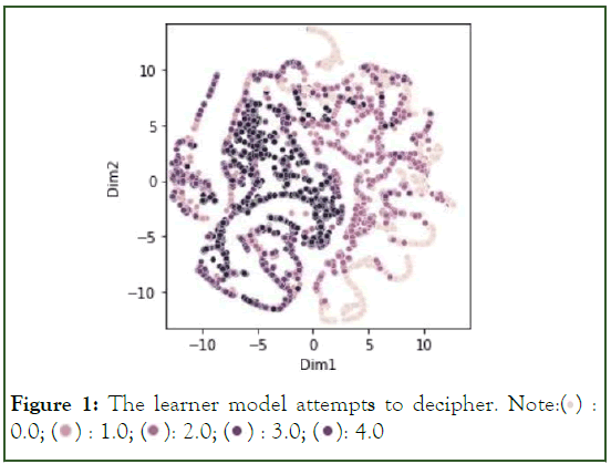
Figure 1: The learner model attempts to decipher. Note: 
 4.0
4.0
The presence of noise and outliers determine the shape and magnitude of the eigenvalue plot. Besides, the limited sample size creates inaccuracy in covariance matrix estimation because the sample covariance matrix is a biased estimator of the actual population covariance matrix and eigenvalue computation. As a consequence, the eigenvalues corresponding to fewer samples are relatively smaller in magnitude [5]. Generally, a real hyperspectral image may contain these factors. In these scenario the so-called thresholding or shrinkage method, and other indices are unable to attain accurate estimation.
The enormous success of machine learning/deep learning in supervised settings motivated us to consider the problem terms of a classification task. It is proven that the eigenvalue of the covariance matrix characterizes the rank-based attribute of the data. Motivated by this fact, we attempt to learn the eigenvalue pattern in a supervised paradigm, where we train the supervised learning method using a large number of eigenvalues with a known number of endmembers. In this scenario, we attempt to learn the eigenvalue pattern from training samples so that the method can infer the endmember number corresponding to an unknown eigenvalue pattern. The learning algorithm/ model once trained with a sufficient number of training observations can uncover the variations within each class sample, and discern the difference between the signal and non-signal components. However, the performance of the supervised learning on the approach relies entirely on the number and quality of the training samples, and the learning algorithm used.
Unlike other standard approaches for counting the endmembers, this work aims to accurately estimate the number of smaller patches, noisy samples, the presence of outliers, and other challenging scenarios. In order to fulfill these aspirations, we require training the machine learning approach on diverse and difficult training examples. To ensure this aforementioned aspect, we created a large number of training samples from the standard real-world HSI datasets, where the ground truth information is also available. However, since the number of such images is relatively limited, we induced Additive White Gaussian Noise (AWGN), performed blurring, cropped random patches, selected a subset of bands, and introduced outliers to these datasets. We computed the covariance matrix from the HSI cube generated from these experiments and recorded the corresponding eigenvalues. Since, the ground truth, i.e. the abundance maps, and the endmember reflectance are known, we could easily obtain the endmember number for these samples. We considered the pair eigenvalue and the number of endmembers for training. However, the size of the eigenvalue vector may not be the same for different reasons- the number of bands corresponding to different images may be different, and band subset selection also creates a different number of bands. However, generally, most real-world images are comprised of a relatively smaller number of endmembers. As a consequence, only the initial 30-40 eigenvalues are sufficient for the prediction task, since the lower eigenvalues represent the noise components. Due to this reason, this work considered the initial k (k<100) eigenvalues so that creating a subset of bands also does not affect the performance significantly. We ensured that the number of eigenvalues is the same for all datasets so that the learning methods do not face any issue regarding the input data dimensionality matching. The work considered the standard supervised setting, where 70% and 30% samples are considered for training and testing, respectively.
The learner/classification model attempts to decipher the eigenvalue pattern and grasp the difference between the signal and non-signal eigenvalues. Hence, we conducted several experiments on standard remotely sensed hyperspectral image datasets. We added Additive White Gaussian Noise (AWGN), performed blurring, and considered small-sized patches. We computed the covariance matrix from all these data experiments and recorded the corresponding eigenvalues. Since these HSI data sets contain well-defined ground truth, we know the number of endmembers in all the samples. Our proposed supervised learning method considers a standard supervised setting where 70% and 30% samples are considered for training and testing, respectively (Figure 1 and 2).
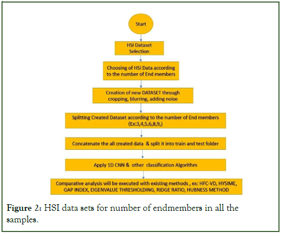
Figure 2: HSI data sets for number of endmembers in all the samples.
We utilized basic, as well as contemporary methods for classifying these eigenvalue patterns. We considered K nearest neighbor, K-Means, Support vector machine, decision tree, Logistic regression, random forest, Artificial neural network, 1D Convolutional neural network, graph Convolutional network, graph attention network, recurrent neural network, etc.
Dataset details
Four real airborne images, namely, Jasper Ridge dataset and urban dataset, were used to perform the experimental analysis. We created training and testing datasets from these datasets.
Jasper ridge: Jasper Ridge is a popularly used for un-mixing analysis. The image has a spatial size of 512 × 614 (Table 1 and Figure 3).
| Created Dataset by adding noise, cropping and blurring from well-known HSI image i.e Jasper ridge, samson, cuprite and urban | Performance | Decision tree | SOFM | BNN | Logistic regression | Random forest classifier | SMOTE + random forest |
XGBoost classifier |
| Accuracy | 77.24% | 62% | 38% | 35% | 81% | 87% | 89% | |
| F1 Score | 16.41% | 79.09% | 87.10% | 88.96% | ||||
| Kappa value | 9.80% | 75.36% | 84.46% | 86.7% |
Table 1: Accuracy comparison through performance index on created dataset from well-known hyper spectral Image.
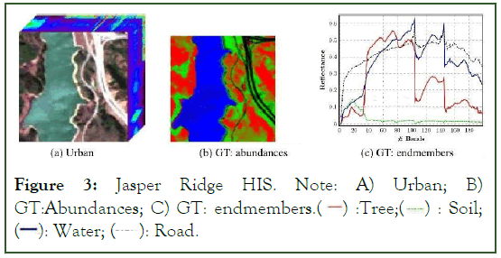
Figure 3: Jasper Ridge HIS. Note: A) Urban; B) GT: Abundances; C) GT: endmembers.  Soil;
Soil;  Road.
Road.
Each pixel is recorded at 224 channels ranging from 380 nm to 2500 nm. The spectral resolution is up to 9.46 nm. Since complex to get the ground truth, we endmembers latent in this data: "#1 Road", "#2 Soil", "#3 Water" and "#4 Tree".
Cuprite: The Cuprite image was captured by hyperspectral unmixing research that covers the Cuprite in Las Vegas, NV, U.S. There are 224 channels, ranging from 370 nm to 2480 nm. After removing the noisy chanels (1–2 and 221–224) and water absorption channels (104aˆ C“113 and 148aˆ C“167), we remain 188 chaAregion of 250 × 190 pixels is considered, where there are 14 types of minerals. Since there are minor differences between variants of similar minerals, we reduce the number of endmembers to 12, which are summarized as follows ”1 Alunite”, ”2 Andradite”, ”3 Buddingtonite”,”4 Dumortierite”, ”5 Kaolinite 1”, ”6 Kaolinite 2”, ”7 Muscovite”, ”8 Montmorillonite”, ”9 Nontronite”, ”10 Pyrope”, ”11 Sphene”, ”12 Chalcedony” (Figure 4).
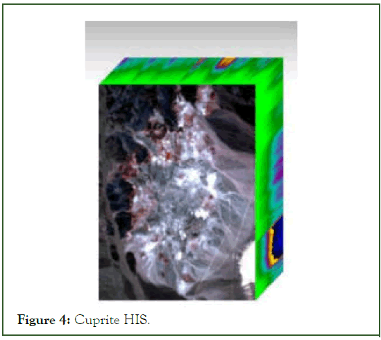
Figure 4: Cuprite HIS.
Hydice urban: Urban is a widely used hyperspectral dataset for unmixing task. The spatial and spectral size of the image is 307×307, and 210, respectively. The 210 spectral bands cover arange of 400 nm to 2500 nm. As per the ground truth, the image comprises of five prominent endmembers, namely, asphalt, grass, tree, roof, and dirt (Figure 5).
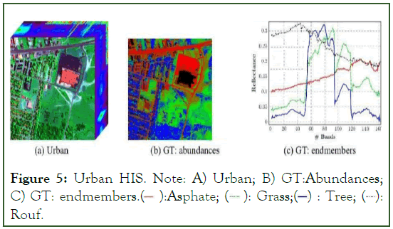
Figure 5: Urban HIS. Note: A) Urban; B) GT: Abundances; C) GT: endmembers.  Rouf.
Rouf.
Samson: Samson is a simple dataset that is available for hyper spectral unmixing. In this image, there are 952 × 952 pixels. Each pixel is recorded at 156 channels covering the wavelengths from 401 nm to 889 nm. The spectral resolution is highly up to 3.13 nm. As the original image is too large, which is very expensive in terms of computational cost, a region of 95 × 95 pixels is used. It starts from the (252,332)th pixel in the original image. This data is not degraded by the blank channel or badly noised channels. Specifically, there are three targets in this image, i.e. "#1 Soil", "#2 Trees" and "#3 Water" respectively (Figure 6).
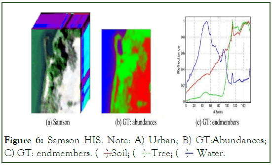
Figure 6: Samson HIS. Note: A) Urban; B) GT: Abundances; C) GT: endmembers.  Water.
Methods compared
Decision trees are a powerful machine learning method for classifying hyperspectral images. They work by recursively splitting the data into smaller subsets based on the values of specific features. The splitting criteria are designed to minimize the impurity of the resulting subsets, which leads to a more accurate classification. Decision trees offer several advantages for hyperspectral image classification.
Simplicity: Decision trees are easy to understand and interpret, making them a good choice for explaining classification decisions.
Robustness: They are relatively robust to noise and outliers in the data.
Feature importance: They provide insights into the relative importance of different features for classification.
Multiple features: They can handle multiple features without requiring complex preprocessing or transformations. However, decision trees also have some limitations.
Overfitting: They may overfit to the training data, leading to poor performance on unseen data.
High-dimensional data: In high-dimensional datasets like hyperspectral images, feature selection becomes crucial to avoid overfitting and improve classification accuracy.
Non-linear relationships: They may struggle to capture complex non-linear relationships between features and the target classes. Overall, decision trees are a valuable tool for hyperspectral image classification, offering a balance of simplicity, interpretability, and robustness. They can be combined with other techniques, such as feature extraction, selection, and ensemble methods, to achieve better classification performance.
Self-Organizing Feature Map (SOM) is a type of artificial neural network that is used for unsupervised learning. SOMs are particularly well-suited for dimensionality reduction, which is the process of reducing the number of features in a dataset to a smaller number of features while preserving as much of the original information as possible. SOMs can be used for hyperspectral image classification by first reducing the dimensionality of the hyperspectral data using a technique such as principal component analysis (PCA). The reduced- dimensionality data is then fed into the SOM, which will learn to map the data onto a lower-dimensional grid of neurons. Each neuron in the grid will be associated with a particular spectral signature, and the neurons that are associated with similar spectral signatures will be located close to each other on the grid. SOMs have been shown to be effective for hyperspectral image classification, especially when combined with other techniques such as dimensionality reduction and feature selection. However, they can be sensitive to noise and may not be able to capture complex relationships between the features and the target classes.
Binarized Neural Networks (BNNs) are a type of artificial neural network that uses binary weights and activations to reduce computational complexity and improve memory efficiency. They have been shown to be effective for hyperspectral image classification, achieving advanced performance on several benchmark datasets.
Hyperspectral image classification of BNNs
Improved accuracy: BNNs can achieve advanced performance on several benchmark datasets.
Computational efficiency: BNNs are significantly less computationally complex than standard neural networks.
Memory efficiency: BNNs require significantly less memory than standard neural networks.
Robustness to noise: BNNs are more robust to noise than standard neural networks.
Scalability: BNNs can be scaled to large datasets by using techniques such as transfer learning and distributed computing. Overall, BNNs are a potential approach for hyperspectral image classification, offering a balance of accuracy, computational efficiency, memory efficiency, and robustness to noise. They are well-suited for a variety of applications, including remote sensing, agriculture, and environmental monitoring.
Logistic regression is a statistical model that predicts the probability of a binary outcome (e.g., class 1 or class 2) given a set of independent variables (e.g., spectral bands). It is a popular choice for hyperspectral image classification because it is simple to implement, interpretable, and can handle high-dimensional data.
Advantages of using logistic regression for hyperspectral image classification
Simplicity: Logistic regression is a relatively simple model to understand and implement.
Interpretability: The weights of the spectral bands in the logistic regression model can be interpreted as the importance of each band in predicting the class label.
Handling high-dimensional data: Logistic regression can handle high-dimensional data such as hyperspectral images without requiring complex preprocessing or transformations. Here are some of the limitations of using logistic regression for hyperspectral image classification.
Sensitivity to noise: Logistic regression can be sensitive to noise in the data.
Limited ability to capture complex relationships: Logistic regression may not be able to capture complex non-linear relationships between the spectral bands and the target classes.
Overfitting: Logistic regression can overfit to the training data, leading to poor performance on unseen data. Overall, logistic regression is a valuable tool for hyperspectral image classification, offering a balance of simplicity, interpretability, and robustness to noise. It can be combined with other techniques, such as feature extraction, selection, and ensemble methods, to achieve better classification performance.
Random forest is a machine learning algorithm that is well- suited for hyperspectral image classification. It is an ensemble method that combines multiple decision trees to make predictions. Each decision tree in the forest is trained on a different subset of the data, and the predictions of the individual trees are then aggregated to make a final prediction. Random forest has been shown to be effective for hyperspectral image classification, achieving state-of-the-art performance on several benchmark datasets. It is a powerful and versatile algorithm that can be used to classify hyperspectral images with high accuracy and robustness to noise.
Advantages of using random forest for hyperspectral image classification
Improved accuracy: Random Forest can achieve advanced performance on several benchmark datasets.
Computational efficiency: Random forest is relatively computationally efficient, as it can be parallelized.
Memory efficiency: Random forest is relatively memory efficient, as it does not require a large amount of memory to store the trained model. Scalability: Random forest can be scaled to large datasets by using techniques such as distributed computing. Overall, random forest is a valuable tool for hyperspectral image classification, offering a balance of accuracy, robustness to noise, interpretability, and scalability. It is well- suited for a variety of applications, including remote sensing, agriculture, and environmental monitoring.
XGBoost, or Extreme Gradient Boosting, is a machine learning algorithm that has become increasingly popular for hyperspectral image classification due to its ability to handle high-dimensional data, its robustness to noise, and its ability to achieve state-of-theart performance. XGBoost is an ensemble method that combines multiple decision trees to make predictions. Each decision tree in the ensemble is trained on a different subset of the data, and the predictions of the individual trees are then aggregated to make a final prediction. Unlike traditional decision trees, XGBoost uses a gradient boosting approach, which involves sequentially adding new trees to the ensemble while minimizing the loss function. XGBoost has been shown to be effective for hyperspectral image classification, achieving state-of-the-art performance on several benchmark datasets. It is a powerful and versatile algorithm that can be used to classify hyperspectral images with high accuracy and robustness to noise.
Some of the advantages of using XGBoost for hyperspectral image classification
Accuracy: XGBoost can achieve state-of-the-art performance on several benchmark datasets.
Handling high-dimensional data: XGBoost can handle high- dimensional data, such as hyperspectral images, without requiring complex preprocessing or transformations.
Robustness to noise: XGBoost is more robust to noise than many other classification algorithms, as the aggregation of the predictions from multiple trees can help to reduce the effects of noise.
Interpretability: XGBoost can be made more interpretable by using techniques such as feature importance measures. Overall, XGBoost is a valuable tool for hyperspectral image classification, offering a balance of accuracy, robustness to noise, interpretability, and scalability. It is well-suited for a variety of applications, including remote sensing, agriculture, and environmental monitoring.
We performed comparative performance assessment with these existing methods on a dataset created by us by introducing noise, performing blurring, and selecting patches from the original data of well-known hyperspectral image.
Conclusion
Hyperspectral imaging technique is a powerful tool for non- destructive assessment of quality in agricultural products. However, the huge amount of information generated by HSI is difficult to process and that limits its use in real time industrial applications. Furthermore, extracting useful information from the high dimensional hyperspectral data containing redundant information is a challenging task. The novelty of this paper is the dataset created totally is new and mixture of different end members from well-known hyperspectral images. We have compared different machine learning algorithm to validate the accuracy which has already given satisfactory result. Machine learning algorithms can play an effective role in analysis of hyperspectral images with high accuracy. Besides, advanced machine learning algorithms like deep learning have found its potential application in hyperspectral image analysis of agricultural products. Since deep learning involves automatic feature learning during the training stage, it has more potential for real time applications than other traditional machine learning algorithms. The scope of lifelong machine learning should be explored further, and its application should be extended to other agricultural crops for quality monitoring. More future work is required in developing Deep learning for reducing the high complexity and optimization task along with estimation of number of end members from our created dataset.
References
- Landgrebe D. Hyperspectral image data analysis. IEEE Signal processing magazine. 2002;19(1):17-28.
- Ma WK, Bioucas-Dias JM, Chan TH, Gillis N, Gader P, Plaza AJ, et al. A signal processing perspective on hyperspectral unmixing: Insights from remote sensing. IEEE Signal Processing Magazine. 2013;31(1):67-81.
- Srivastava MS, Yanagihara H, Kubokawa T. Tests for covariance matrices in high dimension with less sample size. Journal of Multivariate Analysis. 2014;130:289-309.
- Das S, Kundu JN, Routray A. Estimation of number of endmembers in a hyperspectral image using Eigen thresholding. In 2015 Annual IEEE India Conference (INDICON) 2015.
- Das S, Routray A. Covariance similarity approach for semiblind unmixing of hyperspectral image. IEEE Geoscience and Remote Sensing Letters. 2019;16(6):937-941.
- Chang CI, Du Q. Estimation of number of spectrally distinct signal sources in hyperspectral imagery. IEEE Transactions on geoscience and remote sensing. 2004;42(3):608-619.
- Bioucas-Dias JM, Nascimento JM. Hyperspectral subspace identification. IEEE Transactions on Geoscience and Remote Sensing. 2008 Jul 2;46(8):2435-2445.
- Das S, Routray A, Deb AK. Noise robust estimation of number of endmembers in a hyperspectral image by eigenvalue based gap index. In 2016 8th Workshop on Hyperspectral Image and Signal Processing: Evolution in Remote Sensing (WHISPERS) 2016.
Citation: Chakrabarti B (2023) Machine Learning-based Estimation of the Number of Endmembers for Unmixing Hyperspectral Image. J Remote Sens GIS. 12:327.
Copyright: © 2023 Chakrabarti B. This is an open-access article distributed under the terms of the Creative Commons Attribution License, which permits unrestricted use, distribution, and reproduction in any medium, provided the original author and source are credited.
