

Indexed In
- Genamics JournalSeek
- JournalTOCs
- CiteFactor
- RefSeek
- Hamdard University
- EBSCO A-Z
- OCLC- WorldCat
- Publons
- Google Scholar
Useful Links
Share This Page
Journal Flyer

Open Access Journals
- Agri and Aquaculture
- Biochemistry
- Bioinformatics & Systems Biology
- Business & Management
- Chemistry
- Clinical Sciences
- Engineering
- Food & Nutrition
- General Science
- Genetics & Molecular Biology
- Immunology & Microbiology
- Medical Sciences
- Neuroscience & Psychology
- Nursing & Health Care
- Pharmaceutical Sciences
Opinion - (2021) Volume 10, Issue 11
Design and Analysis of Micro Channel Heat Exchanger with Different Geometry Configuration
Balamurugan S*Received: 20-Sep-2021 Published: 03-Nov-2021, DOI: 10.35248/2168-9873.21.10.394
Abstract
In current scenario the surge in fossil fuels prices and demands for cleaner energy sources leads to focus on saving of existing energy usages. Among them heat exchangers are becoming a more viable technology for heat transfer applications. Currently, circular shape channels in heat exchangers dominate commercially than other shape of channels like square, rectangular, trapezoidal etc. However, trapezoidal and rectangular shape channel has some advantage over the circular shape channel. In this project the alteration of circular shape to trapezoidal and rectangular micro channels may increase the overall heat transfer efficiency compare to existing methods. These results are proved in Computational Fluid Dynamics (CFD) and the designing of micro channels are done in Solid Works package.
Keywords
Computational Fluid Dynamics (CFD); Heat exchanging process; Number of Transfer Units (NTU) method
Introduction
Throughout the variety of engineering applications heat exchanger is one of the most usable devices in both domestic and industrial applications [1-10]. Among that device some flub occurs like heat losses happened due to pressure drop, leakages may reduce the performance of heat exchanging process. To avoid these kinds of flubs we may change the design configuration of heat exchangers tubes from its existing geometrical shapes and to workout with same procedures and to gather the results for that new configuration models and then comparison takes place to find the best results [11-20].
Heat exchanger
Heat exchanger is a device used to transfer heat between a solid object and a fluid, or between two or more fluids (Figure 1). The fluids may be separated by a solid wall to prevent mixing or they may be in direct contact. They are widely used in space heating, refrigeration, air conditioning, chemicals, petrochemicals, petroleum refineries, natural-gas processing, and treatment. The classic example of a heat exchanger is found in an internal combustion engine in which a circulating fluid known as engine coolant flows through radiator coils and air flows past the coils, which cools the coolant and heats the incoming air. Another example is the heat sink, which is a passive heat exchanger that transfers the heat generated by an electronic or a mechanical device to a fluid medium, often air or a liquid coolant.

Figure 1: Heat exchanger.
Flow arrangement
There are three primary classifications of heat exchangers according to their flow arrangement. In parallel-flow heat travel in parallel to one another to the other side (Figure 2). In counter-flow heat exchangers the fluids enter the exchanger from opposite ends. The counter current design is the most efficient, in that it can transfer the most heat from the heat transfer medium per unit mass due to the fact that the average temperature difference along any unit length is higher. See counter current exchange. In a cross-flow heat exchanger, the fluids travel roughly perpendicular to one another through the exchanger.

Figure 2: Counter flow-A and Parallel flow–B.
For efficiency, heat exchangers are designed to maximize the surface area of the wall between the two fluids, while minimizing resistance to fluid flow through the exchanger. The exchanger's performance can also be affected by the addition of fins or corrugations in one or both directions, which increase surface area and may channel fluid flow or induce turbulence.
The driving temperature across the heat transfer surface varies with position, but an appropriate means temperature can be defined. In most simple systems this is the "Logarithmic Mean Temperature Difference", (LMTD). Sometimes direct knowledge of the LMTD is not available and the Number of Transfer Units (NTU) method is used.
Types of heat exchangers
Double pipe heat exchangers are the simplest exchangers used in industries. On one hand, these heat exchangers are cheap for both design and maintenance, making them a good choice for small industries (Figures 3 and 4). On the other hand, their low efficiency coupled with the high space occupied in large scales, has led modern industries to use more efficient heat exchangers like shell and tube or plate. However, since double pipe heat exchangers are simple, they are used to teach heat exchanger design basics to students as the fundamental rules for all heat exchangers are the same.

Figure 3: Shell and tube heat exchanger.

Figure 4: Plate heat exchanger.
Shell and tube heat exchanger: Shell and tube heat exchangers consist of series of tubes. One set of these tubes contains the fluid that must be either heated or cooled. The second fluid runs over the tubes that are being heated or cooled so that it can either provide the heat or absorb the heat required. A set of tubes is called the tube bundle and can be made up of several types of tubes: plain, longitudinally finned, etc. Shell and tube heat exchangers are typically used for high-pressure applications (with pressures greater than 30 bar and temperatures greater than 260°C). This is because the shell and tube heat exchangers are robust due to their shape. Several thermal design features must be considered when designing the tubes in the shell and tube heat exchangers: There can be many variations on the shell and tube design. Typically, the ends of each tube are connected to plenums sometimes called water boxes through holes in tube sheets. The tubes may be straight or bent in the shape of U called U-tubes. Using a small tube diameter makes the heat exchanger both economical and compact. However, it is more likely for the heat exchanger to foul up faster and the small size makes mechanical cleaning of the fouling difficult.
To prevail over the fouling and cleaning problems, larger tube diameters can be used. Thus to determine the tube diameter, the available space, cost and fouling nature of the fluids must be considered.
Plate heat exchangers: Another type of heat exchanger is the plate heat exchanger. These exchangers are composed of many thin, slightly separated plates that have very large surface areas and small fluid flow passages for heat transfer. Advances in gasket and brazing technology have made the plate-type heat exchanger increasingly practical. In HVAC applications, large heat exchangers of this type are called plate-and-frame; when used in open loops, these heat exchangers are normally of the gasket type to allow periodic disassembly, cleaning, and inspection. There are many types of permanently bonded plate heat exchangers, such as dip-brazed, vacuum-brazed, and welded plate varieties, and they are often specified for closed-loop applications such as refrigeration. Plate heat exchangers also differ in the types of plates that are used, and in the configurations of those plates. Some plates may be stamped with "chevron", dimpled, or other patterns, where others may have machined fins and grooves.
When compared to shell and tube exchangers, the stackedplate arrangement typically has lower volume and cost. Another difference between the two is that plate exchangers typically serve low to medium pressure fluids, compared to medium and high pressures of shell and tube. A third and important difference is that plate exchangers employ more counter current flow rather than cross current flow, which allows lower approach temperature differences, high temperature changes, and increased efficiencies.
Plate fin heat exchanger: This type of heat exchanger uses "sandwiched" passages containing fins to increase the effectiveness of the unit. The designs include cross flow and counter flow coupled with various fin configurations such as straight fins, offset fins and wavy fins. Plate and fin heat exchangers are usually made of aluminum alloys, which provide high heat transfer efficiency. The material enables the system to operate at a lower temperature difference and reduce the weight of the equipment. Plate and fin heat exchangers are mostly used for low temperature services such as natural gas, helium and oxygen liquefaction plants, air separation plants and transport industries such as motor and aircraft engines.
Pillow plate heat exchanger: A pillow plate exchanger is commonly used in the dairy industry for cooling milk in large direct-expansion stainless steel bulk tanks. The pillow plate allows for cooling across nearly the entire surface area of the tank, without gaps that would occur between pipes welded to the exterior of the tank. The pillow plate is constructed using a thin sheet of metal spot-welded to the surface of another thicker sheet of metal. The thin plate is welded in a regular pattern of dots or with a serpentine pattern of weld lines. After welding the enclosed space is pressurized with sufficient force to cause the thin metal to bulge out around the welds, providing a space for heat exchanger liquids to flow, and creating a characteristic appearance of a swelled pillow formed out of metal.
Fluid heat exchangers: This is a heat exchanger with a gas passing upwards through a shower of fluid often water and the fluid is then taken elsewhere before being cooled. This is commonly used for cooling gases whilst also removing certain impurities, thus solving two problems at once. It is widely used in espresso machines as an energy-saving method of cooling super-heated
Applications
Heat exchangers are widely used for industrial as well as domestic applications. They are present in a majority of equipment’s that we use daily- cars, Air conditioners, refrigerators, heating systems, etc. As far as industrial use is concerned, all installations that use engine, heating mechanism of some kind, heavy machinery need heat exchangers. Heat exchangers not only protect the main equipment, but also make it efficient in usage. This leads to cost savings in short as well as long term. Let us look at various uses of heat exchangers.
Heat exchanger for domestic usage: Air conditioners use two heat exchangers. One sucks the ambient air from the room and passes it through Freon which is the refrigerant used in Air conditioners. This cool air is again sent back to the room where it cools the confined space. The second heat exchanger is meant for Freon itself which tends to heat up in the process of chilling the air. The refrigerator uses a heat exchanger that transfers the heat from inside the refrigerator to the outside. It accomplishes this with the help of a coolant which runs through pipes in the fridge and absorbs heat and ejects it outside. A heating system that protects you from harsh temperatures of the winter season is a big heat exchanger. Your heating system works either by heating water or oil, which is then circulated across the house through pipes. In some cases the heat exchanger’s plate is heated which is then circulated in the house using blowers. Cars use a heat exchanger for cooling the lubricant used in the engine which heats up as the pistons in the engine move at high speed.
Heat exchanger in industrial applications: Power Plants generate steam that rotates the turbine which in turn generates electricity. The steam again makes its way to condense and turns into water. This entire process uses a heat exchanger to convert water into steam and vice versa. Reduction of heat emission: In most of the industrial processes the heat is usually emitted into the open air, but using a heat exchanger particularly economizer can reduce it. The hot air is redirected to an economizer which puts it to use again for the production or industrial process. These way heat exchangers do play a big part in controlling air pollution. Waste water management: The water released as effluent has to be of certain grades and temperature and, heat exchangers help in the process. Hydraulic machinery uses heat exchangers to cool the hydraulic oil, which gets heated up during hydraulic operations. Generators use oil for lubricating and cooling pistons. This oil is cooled by a heat exchanger.
Literature Review
CFD analysis of micro-channel heat exchangers by Karthikeyan V and Sundaram K in 2015
In this project they set an objective was, “Due to the high performance of electronics components, the heat generation is increasing dramatically. Heat dissipation becomes a significant issue for stable operation of components. Micro channels provide very high heat transfer coefficients because of their small diameters. In this study, two dimensional fluid flow and heat transfer in a rectangular micro channel heat sink are analyzed using FLUENT as a solver with water as cooling fluid. With strong literature study, it is found that down to 50 μm of hydraulic diameter, macro scale model can be applicable. Three channels of height 50 μm, 100 μm and 150 μm are considered. The study is mainly focused on Nusselt number and height effects on micro channel thermal performance. The highest temperature is encountered at the heated surface of heat sink immediately above the channel outlet (Figures 5-7). The thermal resistance becomes smaller at the small channel height, indicating that the heat transfer performance can be enhanced at small channel height. Pressure drop becomes more for large channel height and length”. At the end of process they got in CFD results which were the given heat flux and Reynolds number the maximum fluid temperature will occur in the large hydraulic diameter and more pressure drop in 100 μm channel.

Figure 5: Circular shape heat exchanger tubes.

Figure 6: Rectangular tube.

Figure 7: Trapezoidal tube.
Development of micro-heat exchanger with stacked plates using LTCC technology by Vasquez E and Morita l g in 2010
In this segment they took a green ceramic tape micro-heat exchanger was developed using low temperature co-fired ceramics technology (LTCC). The device was designed by using Computational Aided Design software and simulations were made using a Computational Fluid Dynamics package (COSMOL Multiphysis) to evaluate the homogeneity of fluid distribution in the micro channels. Four geometries were proposed and simulated in two and three dimensions to show that geometric details directly affect the distribution of velocity in the micro channel heat exchanger. The simulation results were quite useful for the design of the micro fluidic device. The micro heat exchanger was then constructed using the LTCC technology and is composed of five thermal exchange plates in cross-flow arrangement and two connecting plates, with all plates stacked to form a device with external dimensions of 26 × 26 × 6 mm3. Finally they got a cross flow multi-plate micro-heat exchanger was designed and CFD results. In that the type four (D) had a best behavior of flow distribution when compared with the three other geometries considered.
Design and analysis of a microscale monolithic modular absorption heat pump in 2011
In this segment the first ever conceptualization, design and successful experimental demonstration of a thermally activated micro-scale absorption heat pump for miniaturized or mobile applications is reported here. Several-fold enhancements in coupled heat and mass transfer possible in micro-scale passages remove significant hurdles that have hindered the implementation of thermally activated heat pumps.
Cooling capacities of 100 W – 10 s of kW are possible through minor changes in component geometry. These mass-producible miniaturized systems can be packaged as discrete, distributed hedonically coupled components integrated into buildings. A 300W nominal cooling capacity ammonia- water absorption heat pump with overall dimensions of 200 × 200 ×34 mm and a mass of 7 kg was fabricated and tested over a range of heat sink temperatures from 20 to 35°C with 500-800 W of desorber heat input to yield cooling duties of 136-300 W. As a result they gained the waste heat recovery and upgrade for heat-driven chillers and heating and airconditioning systems, vehicular, marine and refrigerated transport of good, medicines, vaccines and other perishable items are among the applications that could benefit from the absorption system technology developed.
CFD analysis of tube-fin ‘no-frost’ evaporators
The purpose of this paper was to access some aspects of the design of evaporators for house hold refrigeration appliances using Computational Fluid Dynamics (CFD). The evaporators under study are tube-fin ‘no-frost’ heat exchangers with forced convection on the air-side and a staggered tube configuration. The calculation methodology was verified against experimental data for the heat transfer rate, thermal conductance and pressure drop obtained for two evaporators with different geometries. The average errors of the heat transfer rate, thermal rate, thermal conductance and pressure drop were 10%, 3% and 11% respectively. The CFD model was then used to assess the influence of geometric parameters such as the presence and position of the electrical heater coil relative to assess the influence of geometric parameters such as the presence and position of the electrical heater coil relative to the tubes, the influence of configuration and the width of the bypass clearance between the outer edge of the fins and the tube bank for conditions typical of the design of household refrigeration appliances. In the conclusion part the heat transfer increase associated with the use of interrupted fins has been quantified. A heat transfer rate similar to the baseline configuration can be achieved with interrupted fins with 33% less fin surface area and an associated air side pressure drop 15% lower than that obtained in the baseline case.
Performance analysis of shell and tube type heat exchanger under the effect of varied operating conditions
This paper consists of extensive thermal analysis of the effects of severe loading conditions on the performance of the heat exchanger. To serve the purpose a simplified model of shell and tube type heat exchanger has been designed using kern’s method to cool the water from 55 to 45 by using water at room temperature. Then we have carried out steady state thermal analysis on ANSYS 14.0 to justify the design. After that the practical working model of the same has been fabricated using the components of the exact dimensions as derived from the designing. We have tested the heat exchanger under various flow conditions using the insulations of aluminium foil, cotton wool, tape, foam, paper etc. We have also tested the heat exchanger under various ambient temperatures to see its effect on the performance of the heat exchanger. Moreover we have tried to create the turbulence by closing the pump opening and observed its effect on its effectiveness. All these observations along with their discussions have been discussed in detail inside the paper.
On the basis of above study it is clear that a lot of factors affect the performance of the heat exchanger and the effectiveness obtained by the formulas depicts the cumulative effect of all the factors over the performance of the heat exchanger. It may be said that the insulation is a good tool to increase the rate of heat transfer if used properly well below the level of critical thickness. Amongst the used materials the cotton wool and the tape have given the best values of effectiveness. Moreover the effectiveness of the heat exchanger also depends upon the value of turbulence provided. However it is also seen that there does not exists direct relation between the turbulence and effectiveness and effectiveness attains its peak at some intermediate value. The ambient conditions for which the heat exchanger was tested do not show any significant effect over the heat exchanger’s performance.
Heat transfer enhancement in fin and tube heat exchanger - A review
This paper proposed the novel approached toward the heat transfer enhancement of plate and fin heat exchanger using improved fin design facilitating the vortex generation. The vortex generator can be embedded in the plane fin and that too in a low cost with effect the original design and setup of the commonly used heat exchangers. The various design modifications which are implemented and studied numerically and experimentally is been discussed in the paper. Various type of possible and cost effective technique of the heat transfer enhancement were presented in this literature review. It is clear the vortex generator technique is one of the promising approaches of heat transfer enhancement. Lot of work been carried out on various designs and use of simulation software made it easier.
Shell and tube heat exchanger design using CFD tools
In present day shell and tube heat exchanger is the most common type heat exchanger widely used in oil refinery and other large chemical process, because it suits high pressure application. The process in solving simulation consists of modeling and meshing the basic geometry of shell and tube heat exchanger using CFD package ANSYS 13.0. The objective of the project is design of shell and tube heat exchanger with helical baffle and study the flow and temperature field inside the shell using ANSYS software tools. The heat exchanger contains 7 tubes and 600 mm length shell diameter 90 mm. The helix angle of helical baffle will be varied from 0 0 to 200. In simulation will show how the pressure varies in shell due to different helix angle and flow rate. The flow pattern in the shell side of the heat exchanger with continuous helical baffles was forced to be rotational and helical due to the geometry of the continuous helical baffles, which results in a significant increase in heat transfer coefficient per unit pressure drop in the heat exchanger. The heat transfer and flow distribution is discussed in detail and proposed model is compared with increasing baffle inclination angle. The model predicts the heat transfer and pressure drop with an average error of 20%.
Thus the model can be improved. The assumption worked well in this geometry and meshing expects the outlet and inlet region where rapid mixing and change in flow direction takes place. Thus improvement is expected if the helical baffle used in the model should have complete contact with the surface of the shell, it will help in more turbulence across shell side and the heat transfer rate will increase. If different flow rate is taken, it might be help to get better heat transfer and to get better temperature difference between inlet and outlet. Moreover the model has provided the reliable results by considering the standard k-e and standard wall function model, but this model over predicts the turbulence in regions with large normal strain. Thus this model can also be improved by using Nusselt number and Reynolds stress model, but with higher computational theory. Furthermore the enhance wall function are not use in this project, but they can be very useful. The heat transfer rate is poor because most of the fluid passes without the interaction with baffles. Thus the design can be modified for better heat transfer in two ways either the decreasing the shell diameter, so that it will be a proper contact with the helical baffle or by increasing the baffle so that baffles will be proper contact with the shell. It is because the heat transfer area is not utilized efficiently. Thus the design can further be improved by creating cross-flow regions in such a way that flow doesn’t remain parallel to the tubes. It will allow the outer shell fluid to have contact with the inner shell fluid, thus heat transfer rate will increase.
Objective
• To alter the geometrical shape of a heat exchanger circulating tubes like trapezoidal and rectangular shape instead of using circular tubes.
• To collect the material details and select the suitable one for proceeding the design process
• To make a specifications for designing the micro channels and also to derive the formulas and equations for designing micro channels.
• To design that geometrical model using Solid works software with respective dimensions.
• To analyze that models in Computational Fluid Dynamics (CFD) software by giving different inputs like fluid passing temperature, pressure, velocity values.
Micro channel tubes
Existing circular tube: In existing model the company fine tubes offers a range of products specifically meeting the demands and specifications required in the fabrication of shell and tube heat exchangers (Figures 8-17). They design and manufacture tubes for the HX market that fully meet the requirements in terms of price, delivery and specifications. Heat exchanger tubes are used for the cooling, heating or re-heating of fluids, gases, or air in a wide range of industries, such as chemical processing, hydro carbon processing and oil refining, nuclear power generation and aerospace.

Figure 8: Sketching diagram of trapezoidal tube.

Figure 9: Part modeling of trapezoidal tube.

Figure 10: Detailing of trapezoidal tube.

Figure 11: Assembly modelling.

Figure 12: Solid modelling.

Figure 13: Heat exchanger design.

Figure 14: Rectangular channel design.

Figure 15: Trapezoidal channel design.

Figure 16: Static analysis for circular tube.

Figure 17: Thermal analysis for circular tube.
Fine Tubes heat exchanger products can be purchased as seamless, welded or welded redrawn tubes in the following materials like nickel alloys, austenitic stainless steels, duplex, super duplex and super alloys. These high performance tubes are available at dimensions between 12.70 mm and 38.10 mm OD, which covers the majority of the standard sizes used. However, Fine Tubes also specializes in the development and production of small diameter thin wall tubing associated with applications in the aerospace and nuclear industries. Our minimum size here is just 0.98 mm OD with a 0.04 mm wall thickness.
Fine Tubes heat exchanger tubes can be supplied in straight lengths up to 20 m. Completed packages of U-bent and C-formed tubes can be supplied ready to be installed in the tube sheet of shell and tube heat exchangers.
Proposing rectangular tube: The proposing rectangular micro channel tube has nickel alloy material as shown in Figure 6 with proper specification and dimension, which is going to be altering instead of using circular channel. This channel is going to be analyzing in computational fluid dynamics software. In that segments the required inputs are given to take the results output and the comparison process takes place between rectangular and circular channels.
Proposing trapezoidal tube: The proposing trapezoidal micro channel tube has nickel alloy material as shown Figure 7 with proper specification and dimension, which is going to be altering instead of using circular channel. This channel is going to be analyzing in computational fluid dynamics software. In that segments the required inputs are given to take the results output and the comparison process takes place between trapezoidal and circular channels.
Design of heat exchanger tube
Modules of design
Sketch module: A sketch is a rapidly executed freehand drawing that is not usually intended as a finished work. A sketch may serve a number of purposes: It might record something that the artist sees, it might record or develop an idea for later use or it might be used as a quick way of graphically demonstrating an image, idea or principle. Sketches can be made in any drawing medium. The term is most often applied to graphic work executed in a dry medium such as graphite, pencil, charcoal or pastel. But it may also apply to drawings executed in pen and ink, ballpoint pen, water colour and oil paint. The latter two are generally referred to as "water colour sketches" and "oil sketches".
A sculptor might model three-dimensional sketches in clay, plasticine or wax. Sketching is generally a prescribed part of the studies of art students. This generally includes making sketches (croquis) from a live model whose pose changes every few minutes. A "sketch" usually implies a quick and loosely drawn work, while related terms such as study, modello and "preparatory drawing" usually refer to more finished and careful works to be used as a basis for a final work, often in a different medium, but the distinction is imprecise. Under drawing is drawing underneath the final work, which may sometimes still be visible, or can be viewed by modern scientific methods such as X-rays. Most visual artists use, to a greater or lesser degree, the sketch as a method of recording or working out ideas.
The sketchbooks of some individual artists have become very well known, including those of Leonardo da Vinci and Edgar Degas which have become art objects in their own right, with many pages showing finished studies as well as sketches. The term "sketchbook" refers to a book of blank paper on which an artist can draw (or has already drawn) sketches. The book might be purchased bound or might comprise loose leaves of sketches assembled or bound together. The ability to quickly record impressions through sketching has found varied purposes in today's culture. Courtroom sketches record scenes and individuals in law courts. Sketches drawn to help authorities find or identify wanted people are called composite sketches. Street artists in popular tourist areas sketch portraits within minutes.
Part module: Part modeling (or modeling) is a consistent set of principles for mathematical and computer modeling of threedimensional solids. Solid modeling is distinguished from related areas of geometric modeling and computer graphics by its emphasis on physical fidelity. Together, the principles of geometric and solid modeling form the foundation of computer-aided design and in general support the creation, exchange, visualization, animation, interrogation, and annotation of digital models of physical objects. The use of solid modeling techniques allows for the automation of several difficult engineering calculations that are carried out as a part of the design process.
Simulation, planning, and verification of processes such as machining and assembly were one of the main catalysts for the development of solid modeling. More recently, the range of supported manufacturing applications has been greatly expanded to include sheet metal manufacturing, injection molding, welding, pipe routing etc. Beyond traditional manufacturing, solid modeling techniques serve as the foundation for rapid prototyping, digital data archival and reverse engineering by reconstructing solids from sampled points on physical objects, mechanical analysis using finite elements, motion planning and NC path verification, kinematic and dynamic analysis of mechanisms, and so on. A central problem in all these applications is the ability to effectively represent and manipulate three-dimensional geometry in a fashion that is consistent with the physical behavior of real artifacts. Solid modeling research and development has effectively addressed many of these issues, and continues to be a central focus of computeraided engineering.
Solid representation schemes
Based on assumed mathematical properties, any scheme of representing solids is a method for capturing information about the class of semi-analytic subsets of Euclidean space. This means all representations are different ways of organizing the same geometric and topological data in the form of a data structure. All representation schemes are organized in terms of a finite number of operations on a set of primitives. Therefore, the modeling space of any particular representation is finite, and any single representation scheme may not completely suffice to represent all types of solids.
For example, solids defined via combinations of regularized Boolean operations cannot necessarily be represented as the sweep of a primitive moving according to a space trajectory, except in very simple cases. This forces modern geometric modeling systems to maintain several representation schemes of solids and also facilitate efficient conversion between representation schemes. Below is a list of common techniques used to create or represent solid models. Modern modeling software may use a combination of these schemes to represent a solid.
Parameterized primitive instancing: This scheme is based on motion of families of objects, each member of a family distinguishable from the other by a few parameters. Each object family is called a generic primitive, and individual objects within a family are called primitive instances. For example, a family of bolts is a generic primitive, and a single bolt specified by a particular set of parameters is a primitive instance. The distinguishing characteristic of pure parameterized instancing schemes is the lack of means for combining instances to create new structures which represent new and more complex objects. The other main drawback of this scheme is the difficulty of writing algorithms for computing properties of represented solids. A considerable amount of familyspecific information must be built into the algorithms and therefore each generic primitive must be treated as a special case, allowing no uniform overall treatment.
Spatial occupancy enumeration: This scheme is essentially a list of spatial cells occupied by the solid. The cells, also called voxels are cubes of a fixed size and are arranged in a fixed spatial grid (other polyhedral arrangements are also possible but cubes are the simplest). Each cell may be represented by the coordinates of a single point, such as the cell's centroid. Usually a specific scanning order is imposed and the corresponding ordered set of coordinates is called a spatial array. Spatial arrays are unambiguous and unique solid representations but are too verbose for use as 'master' or definitional representations. They can, however, represent coarse approximations of parts and can be used to improve the performance of geometric algorithms, especially when used in conjunction with other representations such as constructive solid geometry.
Cell decomposition: This scheme follows from the combinatoric (algebraic topological) descriptions of solids detailed above. A solid can be represented by its decomposition into several cells. Spatial occupancy enumeration schemes are a particular case of cell decompositions where all the cells are cubical and lie in a regular grid. Cell decompositions provide convenient ways for computing certain topological properties of solids such as its connectedness (number of pieces) and genus (number of holes). Cell decompositions in the form of triangulations are the representations used in 3D finite elements for the numerical solution of partial differential equations. Other cell decompositions such as a Whitney regular stratification or Morse decompositions may be used for applications in robot motion planning.
Boundary representation: In this scheme a solid is represented by the cellular decomposition of its boundary. Since the boundaries of solids have the distinguishing property that they separate space into regions defined by the interior of the solid and the complementary exterior according to the Jordan-Brouwer theorem discussed above, every point in space can unambiguously be tested against the solid by testing the point against the boundary of the solid. Recall that ability to test every point in the solid provides a guarantee of solidity. Using ray casting it is possible to count the number of intersections of a cast ray against the boundary of the solid.
Even numbers of intersections correspond to exterior points, and odd numbers of intersections correspond to interior points. The assumption of boundaries as manifold cell complexes forces any boundary representation to obey disjointedness of distinct primitives, i.e. there are no self-intersections that cause nonmanifold points. In particular, the manifoldness condition implies all pairs of vertices are disjoint, pairs of edges are either disjoint or intersect at one vertex, and pairs of faces are disjoint or intersect at a common edge. Several data structures that are combinatorial maps have been developed to store boundary representations of solids. In addition to planar faces, modern systems provide the ability to store quadrics and NURBS surfaces as a part of the boundary representation. Boundary representations have evolved into a ubiquitous representation scheme of solids in most commercial geometric modelers because of their flexibility in representing solids exhibiting a high level of geometric complexity.
Surface mesh modelling: Similar to boundary representation, the surface of the object is represented. However, rather than complex data structures and NURBS, a simple surface mesh of vertices and edges is used. Surface meshes can be structured (as in triangular meshes in STL files or quad meshes with horizontal and vertical rings of quadrilaterals), or unstructured meshes with randomly grouped triangles and higher level polygons.
Constructive solid geometry: Constructive solid geometry (CSG) connotes a family of schemes for representing rigid solids as Boolean constructions or combinations of primitives via the regularized set operations discussed above. CSG and boundary representations are currently the most important representation schemes for solids. CSG representations take the form of ordered binary trees where non-terminal nodes represent transformations (orientation preserving isometries) or regularized set operations. Terminal nodes are primitive leaves that represent closed regular sets.
The semantics of CSG representations is clear. Each subtree represents set resulting from applying the indicated transformations/ regularized set operations on the set represented by the primitive leaves of the subtree. CSG representations are particularly useful for capturing design intent in the form of features corresponding to material addition or removal (bosses, holes, pockets etc.). The attractive properties of CSG include conciseness, guaranteed validity of solids, computationally convenient Boolean algebraic properties, and natural control of a solid's shape in terms of high level parameters defining the solid's primitives and their positions and orientations. The relatively simple data structure and elegant recursive algorithms have further contributed to the popularity of CSG.
Sweeping: The basic notion embodied in sweeping schemes is simple. A set moving through space may trace or sweep out volume (a solid) that may be represented by the moving set and its trajectory. Such a representation is important in the context of applications such as detecting the material removed from a cutter as it moves along a specified trajectory, computing dynamic interference of two solids undergoing relative motion, motion planning, and even in computer graphics applications such as tracing the motions of a brush moved on a canvas. Most commercial CAD systems provide (limited) functionality for constructing swept solids mostly in the form of a two dimensional cross section moving on a space trajectory transversal to the section. However, current research has shown several approximations of three dimensional shapes moving across one parameter, and even multi-parameter motions.
Parametric and feature-based modelling: Features are defined to be parametric shapes associated with attributes such as intrinsic geometric parameters (length, width, depth etc.), position and orientation, geometric tolerances, material properties, and references to other features. Features also provide access to related production processes and resource models. Thus, features have a semantically higher level than primitive closed regular sets. Features are generally expected to form a basis for linking CAD with downstream manufacturing applications, and also for organizing databases for design data reuse. Parametric feature based modeling is frequently combined with constructive binary solid geometry (CSG) to fully describe systems of complex objects in engineering.
Assembly module: Assembly modeling is a technology and method used by computer-aided design and product visualization computer software systems to handle multiple files that represent components within a product. The components within an assembly are represented as solid or surface models. The designer generally has access to models that others are working on concurrently. For example, several people may be designing one machine that has many parts. New parts are added to an assembly model as they are created. Each designer has access to the assembly model, while a work in progress, and while working in their own parts. The design evolution is visible to everyone involved.
Depending on the system, it might be necessary for the users to acquire the latest versions saved of each individual components to update the assembly. The individual data files describing the 3D geometry of individual components are assembled together through a number of sub-assembly levels to create an assembly describing the whole product. All CAD and CPD systems support this form of up construction. Some systems, via associative copying of geometry between components also allow top-down method of design. Components can be positioned within the product assembly using absolute coordinate placement methods or by means of mating conditions.
Mating conditions are definitions of the relative position of components between each other; for example alignment of axis of two holes or distance of two faces from one another. The final position of all components based on these relationships is calculated using a geometry constraint engine built into the CAD or visualization package. The importance of assembly modeling in achieving the full benefits of PLM has led to ongoing advances in this technology. These include the use of lightweight data structures such as JT that allow visualization of and interaction with large amounts of product data, direct interface to between Digital Mock ups and PDM systems and active digital mock up technology that unites the ability to visualize the assembly mock up with the ability to measure, analyze, simulate, design and redesign.
Detailing: Detail drawings provide a detailed description of the geometric form of a part of an object such as a building, bridge, tunnel, machine, plant and so on. They tend to be large-scale drawings that show in detail parts that may be included in less detail on general arrangement drawings. Detail drawings may be used to demonstrate compliance with regulations and other requirements, to provide information about assembly and the junctions between components, to show construction details, detailed form and so on, that would not be possible to include on more general drawings. They may include dimensions, tolerances, notation, symbols and specification information, but this should not duplicate information included in separate specifications as this can become contradictory and may cause confusion. They may consist of two dimensional orthogonal projections showing plans, sections and elevations and may be drawn to scale by hand, or prepared using Computer Aided Design (CAD) software. However, increasingly, building information modeling (BIM) is being used to create detailed 3 dimensional representations of buildings and their components. Detail drawings may be confused with ‘detailed design drawings’ which might describe the drawings produced during the detailed design stage, (sometimes referred to as 'developed design' or 'definition'). Detailed design is the process developing the design so that it is dimensionally correct and coordinate, describing all the main components of the building and how they fit together. Not all drawings produced during this stage will necessarily be detail drawings. They are also distinct from the definition of ‘working drawings’ which provide dimensioned, graphical information that can be used by a contractor to construct the works, by suppliers to fabricate components of the works or to assemble or install components. Again, not all working drawings will necessarily be detail drawings.
Modeling software
In this phase the design process made with the use of solid works software. The brief explanation for this software is in the following paragraphs.
Solid works: Solid Works is a solid modeling computer-aided design (CAD) and computer-aided engineering (CAE) computer program that runs on Microsoft Windows. Solid Works is published by Dassault Systèmes. According to the publisher, over two million engineers and designers at more than 165,000 companies were using solid Works as of 2013. Also according to the company, fiscal year 2011-2012 revenue for solid works totaled $483 million. Solid Works Corporation was founded in December 1993 by Massachusetts Institute of Technology graduate Jon Hirschtick. Hirschtick used $1 million he had made while a member of the MIT Blackjack Team to set up the company.
Initially based in Waltham, Massachusetts, United States, Hirschtick recruited a team of engineers with the goal of building 3D CAD software that was easy-to-use, affordable, and available on the Windows desktop. Operating later from Concord, Massachusetts, solid works released its first product solid works 95, in November 1995. In 1997 Dassault, best known for its CATIA CAD software, acquired Solid Works for $310 million in stock. Jon Hirschtick stayed on board for the next 14 years in various roles. Under his leadership, Solid Works grew to a $100 million revenue company.
Solid Works currently markets several versions of the Solid Works CAD software in addition to e-Drawings, a collaboration tool, and Draft Sight, a 2D CAD product. Solid Works was headed by John McEleney from 2001 to July 2007 and Jeff Ray from 2007 to January 2011. The current CEO is Gian Paolo Bassi from Jan 2015. Gian Paolo Bassi replaces Bertrand Sicot, who is promoted Vice President Sales of Dassault Systèmes’ Value Solutions sales channel.
Modeling technology: Solid Works is a solid modeler, and utilizes a parametric feature-based approach to create models and assemblies. The software is written on Para solid-kernel. Parameters refer to constraints whose values determine the shape or geometry of the model or assembly. Parameters can be either numeric parameters, such as line lengths or circle diameters, or geometric parameters, such as tangent, parallel, concentric, horizontal or vertical, etc.
Numeric parameters can be associated with each other through the use of relations, which allow them to capture design intent. Design intent is how the creator of the part wants it to respond to changes and updates. For example, you would want the hole at the top of a beverage can to stay at the top surface, regardless of the height or size of the can. Solid Works allows the user to specify that the hole is a feature on the top surface, and will then honor their design intent no matter what height they later assign to the can.
Features refer to the building blocks of the part. They are the shapes and operations that construct the part. Shape-based features typically begin with a 2D or 3D sketch of shapes such as bosses, holes, slots, etc. This shape is then extruded or cut to add or remove material from the part. Operation-based features are not sketch-based, and include features such as fillets, chamfers, shells, applying draft to the faces of a part, etc.
Building a model in Solid Works usually starts with a 2D sketch (although 3D sketches are available for power users). The sketch consists of geometry such as points, lines, arcs, conics (except the hyperbola), and splines. Dimensions are added to the sketch to define the size and location of the geometry. Relations are used to define attributes such as tangency, parallelism, perpendicularity, and concentricity.
The parametric nature of Solid Works means that the dimensions and relations drive the geometry, not the other way around. The dimensions in the sketch can be controlled independently, or by relationships to other parameters inside or outside of the sketch. In an assembly, the analog to sketch relations are mates. Just as sketch relations define conditions such as tangency, parallelism, and concentricity with respect to sketch geometry, assembly mates define equivalent relations with respect to the individual parts or components, allowing the easy construction of assemblies. Solid Works also includes additional advanced mating features such as gear and cam follower mates, which allow modeled gear assemblies to accurately reproduce the rotational movement of an actual gear train. Finally, drawings can be created either from parts or assemblies. Views are automatically generated from the solid model, and notes, dimensions and tolerances can then be easily added to the drawing as needed.
File format: Solid Works files (previous to version 2015) use the Microsoft Structured Storage file format. This means that there are various files embedded within each SLDDRW (drawing files), SLDPRT (part files), SLDASM (assembly files) file, including preview bitmaps and metadata sub-files. Various third-party tools (COM Structured Storage) can be used to extract these sub-files, although the sub files in many cases use proprietary binary file formats.
Solid works market: DS Solid Works Corp has sold over 1.5 million licenses of solid works worldwide. This includes a large proportion of educational licenses. The Sheffield Telegraph comments that Solid Works is the world's most popular CAD software. Its user base ranges from individuals to large corporations, and covers a very wide cross-section of manufacturing market segments. Commercial sales are made through an indirect channel, which includes dealers and partners throughout the world. Solid works also partners with third party developers to add functionality in niche market applications like finite element analysis, circuit layout, tolerance checking, etc. Solid Works has also licensed its 3D modeling capabilities to other CAD software vendors, notably ANVIL.
The above figures are showing the existing circular geometrical heat exchanger tubes with the structural and thermal analysis results
Specification for micro channels
Specification for circular shape channel:
Length of the channel, L=58.54 mm
Diameter of the circular tube (internal), d1=ᶲ 0.22 mm
Diameter of the circular tube (external), d2=ᶲ 0.24 mm
Specification for rectangular shape channel:
Length of the channel, L= 58.54 mm
Height of the channel, h=0.25 mm
Breadth of the channel, b= 0.35 mm
Specification for trapezoidal shape channel:
Length of the channel, L= 58.54 mm
Height of the channel, h=0.25 mm
Breadth of the channel, b=0.35 m
Breadth of the channel, b2=0.32 mm
Materials usage for micro channels
Nickel alloy: Nickel alloys are used extensively because of their corrosion resistance, high temperature strength and their special magnetic and thermal expansion properties. Nickel chromium base alloys are used extensively in applications where heat resistance and/or corrosion resistance is required. In some members of the group, where conditions are less demanding, some nickel is replaced by iron to decrease the overall cost. Metals fail at high temperatures by both oxidation (scaling) and through a loss in strength. Alloys in this class are designed to resist failure from both of these mechanisms. Nickel alloys are not suitable for high temperature sulphur rich environments. Where corrosion resistance is significant, molybdenum is used as an alloying addition in nickel chromium based alloys. These groups of alloys are frequently sold under trade name specifications but most are listed in the Unified Numbering System. The more recent nickel chromium base alloys in these groups also have a wide range of ancillary elements added to give special proper ties - some of these can be quite complicated and require very close control over composition and heat treatment. Nickel is a chemical element with symbol Ni and atomic number 28. It is a silvery-white lustrous metal with a slight golden tinge. Nickel belongs to the transition metals and is hard and ductile. Pure nickel, powdered to maximize the reactive surface area, shows a significant chemical activity, but larger pieces are slow to react with air under standard conditions because an oxide layer forms on the surface and prevents further corrosion (passivation). Even so, pure native nickel is found in Earth's crust only in tiny amounts, usually in ultramafic rocks, and in the interiors of larger nickel–iron meteorites that were not exposed to oxygen when outside Earth's atmosphere. Meteoric nickel is found in combination with iron, a reflection of the origin of those elements as major end products of supernova nucleosynthesis. An iron– Use of nickel (as a natural meteoric nickel–iron alloy) has been traced as back as 3500 BCE. Nickel was first isolated and classified as a chemical element in 1751 by Axel Fredrik Cronstedt, who initially mistook the ore for a copper mineral, in the cobalt mines of Los, Hälsingland, Sweden. The element's name comes from a mischievous sprite of German miner mythology, Nickel (similar to Old Nick), that personified the fact that copper-nickel ores resisted refinement into copper. An economically important source of nickel is the iron ore limonite, which often contains 1–2% nickel. Nickel's other important ore minerals include garnierite, and pentlandite. Major production sites include the Sudbury region in Canada (which is thought to be of meteoric origin), New Caledonia in the Pacific, and Norilsk in Russia. Nickel is slowly oxidized by air at room temperature and is considered corrosion-resistant. Historically, it has been used for plating iron and brass, coating chemistry equipment, and manufacturing certain alloys that retain a high silvery polish, such as German silver. About 9% of world nickel production is still used for corrosion-resistant nickel plating. Nickel-plated objects sometimes provoke nickel allergy. Nickel has been widely used in coins, though its rising price has led to some replacement with cheaper metals in recent years.
Nickel is one of four elements (iron, cobalt, nickel, and gadolinium) that are ferromagnetic approximately temperature. Alnico permanent magnets based partly on nickel are of intermediate strength between iron-based permanent magnets and rare-earth magnets. The metal is valuable in modern times chiefly in alloys; about 68% of world production is used in stainless steel. A further 10% is used for nickel-based and copper-based alloys, 7% for alloy steels, 3% in foundries, 9% in plating and 4% in other applications, including the fast-growing battery sector. As a compound, nickel has a number of niche chemical manufacturing uses, such as a catalyst for hydrogenation, cathodes for batteries, pigments and metal surface treatments. Nickel is an essential nutrient for some microorganisms and plants that have enzymes with nickel as an active site.
Physical properties: Nickel is a silvery-white metal with a slight golden tinge that takes a high polish. It is one of only four elements that are magnetic at or near room temperature, the others being iron, cobalt and gadolinium. Curie temperature is 355°C (671°F) meaning that bulk nickel is non-magnetic above this temperature. The unit cell of nickel is a face-centered cube with the lattice parameter of 0.352 nm, giving an atomic radius of 0.124 nm. This crystal structure is stable to pressures of at least 70 GPa. Nickel belongs to the transition metals and is hard and ductile (Figure 18).

Figure 18: Nickel alloy bar.
Austenitic stainless steels: Austenitic stainless steel is a specific type of stainless steel alloy. Stainless steels may be classified by their crystalline structure into three main types: austenitic, ferritic and martensitic. 300 Series austenitic stainless steel has austenite as its primary phase (face centered cubic crystal). These are alloys containing chromium and nickel, and sometimes molybdenum and nitrogen, structured around the Type 302 composition of iron, 18% chromium, and 8% nickel. 200 Series austenitic stainless steels replace the majority of their nickel content with manganese to reduce cost. Austenitic steels are not hardenable by heat treatment. The most familiar stainless steel is probably SAE 304 stainless steel, also called 18/8 or A2 stainless steel. Type 304 surgical stainless steel is austenitic steel containing 18–20% chromium and 8–10% nickel. Alloy 20 (Carpenter 20) is an austenitic stainless steel possessing excellent resistance to hot sulfuric acid and many other aggressive environments which would readily attack type 316 stainless. This alloy exhibits superior resistance to stress-corrosion cracking in boiling 20–40% sulfuric acid. Alloy 20 has excellent mechanical properties and the presence of niobium in the alloy minimizes the precipitation of carbides during welding. Austenitic stainless steel can be tested by nondestructive testing using the dye penetrant inspection method but not the magnetic particle inspection method. Eddy-current testing may also be used. It is the primary stainless steel used in aviation construction. Chemical and steel industry-applicable grades are SAE steel grades 308 L, 316 L. "L" denotes a carbon percentage less than 0.03%, mostly used for corrosion heat resistance and reducing sensitivity to chromium carbide formation. Another grade, 312, is used for dissimilar steel welding, also known as universal alloy steel as unknown composition steels can be welded. For high temperature applications at greater than 600°C, grades 309 and 310 are preferred. Grade 316 is alloyed with molybdenum (~2–3%) for high-temperature strength, pitting and crevice corrosion resistance. Stainless steels may be classified by their crystalline structure into three main types: austenitic, ferritic and martensitic. Martensitic stainless steels can be high or low-carbon steels built around the Type 410 composition of iron, 12% chromium, and up to 1.2% carbon. They are usually tempered and hardened. Tempered martensite gives steel good hardness and high toughness; used largely for medical tools (scalpels, razors and internal clamps). Untempered martensite is low in toughness and therefore brittle. The characteristic body-centered tetragonal martensite microstructure was first observed by German microscopist Adolf Martens around 1890. In 1912, Elwood Haynes applied for a U.S. patent on a martensitic stainless steel alloy. This patent was not granted until 1919. Martensitic stainless steel can be nondestructively tested using the magnetic particle inspection method, unlike austenitic stainless steel. Also in 1912, Harry Brearley of the Brown-Firth research laboratory in Sheffield, England, while seeking a corrosion-resistant alloy for gun barrels, discovered and subsequently industrialized a martensitic stainless steel alloy. The discovery was announced two years later in a January 1915 newspaper article in The New York Times. Brearly applied for a U.S. patent during 1915. This was later marketed under the "Staybrite" brand by Firth Vickers in England and was used for the new entrance canopy for the Savoy Hotel in 1929 in London.
Duplex: Duplex stainless steels are called “duplex” because they have a two-phase microstructure consisting of grains of ferritic and austenitic stainless steel. The picture shows the yellow austenitic phase as “islands” surrounded by the blue ferritic phase. When duplex stainless steel is melted it solidifies from the liquid phase to a completely ferritic structure. As the material cools to room temperature, about half of the ferritic grains transform to austenitic grains “islands”. The result is a microstructure of roughly 50% austenite and 50% ferrite. The idea of duplex stainless steels dates back to the 1920s with the first cast being made at Avesta in Sweden in 1930. However, it is only in the last 30 years that duplex steels have begun to “take off” in a significant way (Figure 19).

Figure 19: Duplex made plates.
The standard austenitic steels like 304 (1.4301) and ferritic steels like 430 are relatively easy to make and to fabricate. As their names imply, they consist mainly of one phase, austenite or ferrite. These types are fine for a wide range of applications: ability in thick sections, poor low temperature toughness. In addition, the high nickel content of the austenitic types leads to price volatility which is unwelcome to many end users. The duplex structure gives this family of stainless steels a combination of attractive properties:
1. Strength: Duplex stainless steels are about twice as strong as regular austenitic or ferritic stainless steels.
2. Toughness and ductility: Duplex stainless steels have significantly better toughness and ductility than ferritic grades; however, they do not reach the excellent value of austenitic steels.
3. Corrosion resistance: As with all stainless steels, corrosion resistance depends mostly on the composition of the stainless steel. For chloride pitting and crevice corrosion resistance, their chromium, molybdenum and nitrogen content are most important. Duplex stainless steel grades have a range of corrosion resistance, similar to the range for austenitic stainless steels, i.e. from Type 304 or 316 (e.g. LDX 2101©) to 6% molybdenum (e.g. SAF 2507©) stainless steels.
4. Stress corrosion cracking resistance: Duplex stainless steels show very good stress corrosion cracking (SCC) resistance, a property they have “inherited” from the ferritic side. SCC can be a problem under certain circumstances (chlorides, humidity and elevated temperature) for standard austenitics such 306.
5. Cost: Duplex stainless steels have lower nickel and molybdenum contents than their austenitic counterparts of similar corrosion resistance. Due to the lower alloying content, duplex stainless steels can be lower in cost, especially in times of high alloy surcharges. Additionally, it may often be possible to reduce the section thickness of duplex stainless steel, due to its increased yield strength compared to austenitic stainless steel. The combination can lead to significant cost and weight savings compared to a solution in austenitic stainless steels.
Formulas and equations
Conduction: The rate of heat conduction is proportional to the area measured normal to the direction of heat flow, and to the temperature gradient in that direction. The formula for conduction is given in below charts.
Q=-kA αT
Convection: The heat flux is directionally proportional to the heat transfer and inversely proportional to the area of respective device. The formula for convection is given in below chart.
q=Q/A
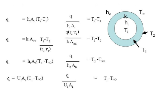
Heat transfer coefficient
Analysis of heat exchanger tube
Mode of analysis
Engineering analysis involves the application of scientific analytic principles and processes to reveal the properties and state of a system, device or mechanism under study. Engineering analysis is decomposition. It proceeds by separating the engineering design into the mechanisms of operation or failure, analyzing or estimating each component of the operation or failure mechanism in isolation, and re-combining the components according to basic physical principles and natural laws.
Modal analysis: Modal analysis is the study of the dynamic properties of systems in the frequency domain. A typical example would be testing structures under vibrational excitation. Modal analysis is the field of measuring or calculating and analyzing the dynamic response of structures and/or fluids or other systems during excitation. Examples would include measuring the vibration of a car's body when it is attached to an electromagnetic shaker, analysis of unforced vibration response of vehicle suspension or the noise pattern in a room when excited by a loudspeaker. Modern day experimental modal analysis systems are composed of sensors such as transducers (typically accelerometers, load cells) or noncontact via a Laser micrometer or stereo photogrammetric data acquisition system and an analog-to-digital converter front end (to digitize analog instrumentation signals) and host PC (personal computer) to view the data and analyze it. Classically this was done with a SIMO (single-input, multiple-output) approach, that is, one excitation point, and then the response is measured at many other points. In the past a hammer survey, using a fixed accelerometer and a roving hammer as excitation, gave a MISO (multiple-input, single-output) analysis, which is mathematically identical to SIMO, due to the principle of reciprocity. In recent years MIMO (multiinput, multiple-output) have become more practical, where partial coherence analysis identifies which part of the response comes from which excitation source. Using multiple shakers leads to a uniform distribution of the energy over the entire structure and a better coherence in the measurement. A single shaker may not effectively excite all the modes of a structure. Typical excitation signals can be classed as impulse, broadband, swept sine, chirp, and possibly others. Each has its own advantages and disadvantages. The analysis of the signals typically relies on Fourier analysis. The resulting transfer function will show one or more resonances, whose characteristic mass, frequency and damping can be estimated from the measurements. The animated display of the mode shape is very useful to NVH (noise, vibration, and harshness) engineers. The results can also be used to correlate with finite element analysis normal mode solutions.
Static analysis: Static analysis, static projection, or static scoring is a simplified analysis wherein the effect of an immediate change to a system is calculated without regard to the longer-term response of the system to that change. If the short-term effect is then extrapolated to the long term, such extrapolation is inappropriate. It’s opposite, dynamic analysis or dynamic scoring, is an attempt to take into account how the system is likely to respond to the change over time. One common use of these terms is budget policy in the United States, although it also occurs in many other statistical disputes. A famous example of extrapolation of static analysis comes from overpopulation theory. Starting with Thomas Malthus at the end of the 18th century, various commentators have projected some short-term population growth trend for years into the future, resulting in the prediction that there would be disastrous overpopulation within a generation or two. Malthus himself essentially claimed that British society would collapse under the weight of overpopulation by 1850, while during the 1960s the book The Population Bomb made similar dire predictions for the US by the 1980s. For economic policy discussions, predictions that assume no significant change of behavior in response to change in incentives are often termed static projection (and in the US Congressional Budget Office, "static scoring"). When applied to dynamically responsive systems, static analysis improperly extrapolated tends to produce results that are not only incorrect but opposite in direction to what was predicted, as shown in the following applications.
Thermal analysis: Thermal analysis is a branch of materials science where the properties of materials are studied as they change with temperature. Several methods are commonly used – these are distinguished from one another by the property which is measured:
• Dielectric Thermal Analysis (DEA): Dielectric permittivity and loss factor
• Differential Thermal Analysis (DTA): Temperature difference vs. temperature or time
• Differential Scanning Calorimetry (DSC): Heat flow changes vs. temperature or time
• Dilatometry (DIL): Volume changes with temperature change
• Dynamic Mechanical Analysis (DMA or DMTA): Measures storage modulus (stiffness) and loss modulus (damping) vs. temperature, time and frequency
• Evolved Gas Analysis (EGA): Analysis of gases evolved during heating of a material, usually decomposition products
• Laser Flash Analysis (LFA): Thermal diffusivity and thermal conductivity
• Thermo Gravimetric Analysis (TGA): Mass change vs. temperature or time
• Thermo Mechanical Analysis (TMA): Dimensional changes vs. temperature or time
• Thermo Optical Analysis (TOA): Optical properties
Simultaneous thermal analysis (STA) generally refers to the simultaneous application of Thermogravimetry (TGA) and differential scanning calorimetry (DSC) to one and the same sample in a single instrument. The test conditions are perfectly identical for the TGA and DSC signals (same atmosphere, gas flow rate, vapor pressure of the sample, heating rate, thermal contact to the sample crucible and sensor, radiation effect, etc.). The information gathered can even be enhanced by coupling the STA instrument to an Evolved Gas Analyzer (EGA) like Fourier transform infrared spectroscopy (FTIR) or mass spectrometry (MS). Other, less common, methods measure the sound or light emission from a sample, or the electrical discharge from a dielectric material, or the mechanical relaxation in a stressed specimen. The essence of all these techniques is that the sample's response is recorded as a function of temperature (and time). It is usual to control the temperature in a predetermined way - either by a continuous increase or decrease in temperature at a constant rate (linear heating/cooling) or by carrying out a series of determinations at different temperatures (stepwise isothermal measurements). More advanced temperature profiles have been developed which use an oscillating (usually sine or square wave) heating rate (Modulated Temperature Thermal Analysis) or modify the heating rate in response to changes in the system's properties (Sample Controlled Thermal Analysis). In addition to controlling the temperature of the sample, it is also important to control its environment (e.g. atmosphere). Measurements may be carried out in air or under an inert gas (e.g. nitrogen or helium). Reducing or reactive atmospheres have also been used and measurements are even carried out with the sample surrounded by water or other liquids. Inverse gas chromatography is a technique which studies the interaction of gases and vapors with a surface - measurements are often made at different temperatures so that these experiments can be considered to come under the auspices of Thermal Analysis. Atomic force microscopy uses a fine stylus to map the topography and mechanical properties of surfaces to high spatial resolution. By controlling the temperature of the heated tip and/or the sample a form of spatially resolved thermal analysis can be carried out. Thermal analysis is also often used as a term for the study of heat transfer through structures. Many of the basic engineering data for modelling such systems comes from measurements of heat capacity and thermal conductivity.
Dynamic analysis: Dynamic mechanical analysis (abbreviated DMA, also known as dynamic mechanical spectroscopy) is a technique used to study and characterize materials. It is most useful for studying the viscoelastic behavior of polymers. A sinusoidal stress is applied and the strain in the material is measured, allowing one to determine the complex modulus. The temperature of the sample or the frequency of the stress are often varied, leading to variations in the complex modulus; this approach can be used to locate the glass transition temperature of the material, as well as to identify transitions corresponding to other molecular motions. One important application of DMA is measurement of the glass transition temperature of polymers. Amorphous polymers have different glass transition temperatures, above which the material will have rubbery properties instead of glassy behavior and the stiffness of the material will drop dramatically with an increase in viscosity. At the glass transition, the storage modulus decreases dramatically and the loss modulus reaches a maximum. Temperature-sweeping DMA is often used to characterize the glass transition temperature of a material. Varying the composition of monomers and crosslinking can add or change the functionality of a polymer that can alter the results obtained from DMA. An example of such changes can be seen by blending ethylene-propylene-diene monomer (EPDM) with styrene-butadiene rubber (SBR) and different crosslinking or curing systems. Nair et al. abbreviate blends as E0S, E20S, etc., where E0S equals the weight percent of EPDM in the blend and S denotes sulfur as the curing agent. Increasing the amount of SBR in the blend decreased the storage modulus due to intermolecular and intra molecular interactions that can alter the physical state of the polymer. Within the glassy region, EPDM shows the highest storage modulus due to stronger intermolecular interactions (SBR has more steric hindrance that makes it less crystalline). In the rubbery region, SBR shows the highest storage modulus resulting from its ability to resist intermolecular slippage. When compared to sulfur, the higher storage modulus occurred for blends cured with dicumylperoxide (DCP) because of the relative strengths of C-C and C-S bonds. Incorporation of reinforcing fillers into the polymer blends also increases the storage modulus at an expense of limiting the loss tangent peak height. DMA can also be used to effectively evaluate the miscibility of polymers. The E40S blend had a much broader transition with a shoulder instead of a steep drop-off in a storage modulus plot of varying blend ratios, indicating that there are areas that are not homogeneous.
Analysing software
In this phase the analysing process made with the use of computational fluid dynamics software. The brief explanation for this software is in the following paragraphs.
Computational fluid dynamics (CFD): It is a branch of fluid mechanics that uses numerical analysis and data structures to solve and analyze problems that involve fluid flows. Computers are used to perform the calculations required to simulate the interaction of liquids and gases with surfaces defined by boundary conditions. With high-speed supercomputers, better solutions can be achieved. Ongoing research yields software that improves the accuracy and speed of complex simulation scenarios such as transonic or turbulent flows. Initial experimental validation of such software is performed using a wind tunnel with the final validation coming in full-scale testing, e.g. flight tests. The fundamental basis of almost all CFD problems is the Navier–Stokes equations, which define many singlephase (gas or liquid, but not both) fluid flows. These equations can be simplified by removing terms describing viscous actions to yield the Euler equations. Further simplification, by removing terms describing vorticity yields the full potential equations. Finally, for small perturbations in subsonic and supersonic flows (not transonic or hypersonic) these equations can be linearized to yield the linearized potential equations. Historically, methods were first developed to solve the linearized potential equations. Twodimensional (2D) methods, using conformal transformations of the flow about a cylinder to the flow about an airfoil were developed in the 1930s. One of the earliest type of calculations resembling modern CFD are those by Lewis Fry Richardson, in the sense that these calculations used finite differences and divided the physical space in cells. Although they failed dramatically, these calculations, together with Richardson's book "Weather prediction by numerical process", set the basis for modern CFD and numerical meteorology. In fact, early CFD calculations during the 1940s using ENIAC used methods close to those in Richardson's 1922 book.
The computer power available paced development of threedimensional methods. Probably the first work using computers to model fluid flow, as governed by the Navier-Stokes equations, was performed at Los Alamos National Lab, in the T3 group. This group was led by Francis H. Harlow, who is widely considered as one of the pioneers of CFD. From 1957 to late 1960s, this group developed a variety of numerical methods to simulate transient two-dimensional fluid flows, such as Particle-in-cell method (Harlow, 1957), Fluid-in-cell method (Gentry, Martin and Daly, 1966), Vorticity stream function method (Jake Fromm, 1963) and Marker-and-cell method (Harlow and Welch, 1965). Fromm's vorticity-stream-function method for 2D, transient, incompressible flow was the first treatment of strongly contorting incompressible flows in the world. The first paper with three-dimensional model was published by John Hess and A.M.O. Smith of Douglas Aircraft in 1967. This method discretized the surface of the geometry with panels, giving rise to this class of programs being called Panel Methods. Their method itself was simplified, in that it did not include lifting flows and hence was mainly applied to ship hulls and aircraft fuselages. The first lifting Panel Code (A230) was described in a paper written by Paul Rubbert and Gary Saaris of Boeing Aircraft in 1968. In time, more advanced three-dimensional Panel Codes were developed at Boeing (PANAIR, A502), Lockheed (Quadpan), Douglas (HESS), McDonnellAircraft (MACAERO), NASA (PMARC) and Analytical Methods (WBAERO, USAERO and VSAERO). Some (PANAIR, HESS and MACAERO) were higher order codes, using higher order distributions of surface singularities, while others (Quadpan, PMARC, USAERO and VSAERO) used single singularities on each surface panel. The advantage of the lower order codes was that they ran much faster on the computers of the time. Its sister code, USAERO is an unsteady panel method that has also been used for modeling such things as high speed trains and racing yachts. The NASA PMARC code from an early version of VSAERO and a derivative of PMARC, named CMARC is also commercially available. In the two-dimensional realm, a number of Panel Codes have been developed for airfoil analysis and design. The codes typically have a boundary layer analysis included, so that viscous effects can be modeled. Professor Richard Eppler of the University of Stuttgart developed the PROFILE code, partly with NASA funding, which became available in the early 1980s. This was soon followed by MIT Professor Mark Drela's XFOIL code. Both PROFILE and XFOIL incorporate two-dimensional panel codes, with coupled boundary layer codes for airfoil analysis work. PROFILE uses a conformal transformation method for inverse airfoil design, while XFOIL has both a conformal transformation and an inverse panel method for airfoil design. An intermediate step between Panel Codes and Full Potential codes were codes that used the Transonic Small Disturbance equations. In particular, the three-dimensional WIBCO code, developed by Charlie Boppe of Grumman Aircraft in the early 1980s has seen heavy use. Developers turned to Full Potential codes, as panel methods could not calculate the nonlinear flow present at transonic speeds. The first description of a means of using the Full Potential equations was published by Earll Murman and Julian Cole of Boeing in 1970. Frances Bauer, Paul Garabedian and David Korn of the Courant Institute at New York University (NYU) wrote a series of two-dimensional Full Potential airfoil codes that were widely used, the most important being named Program H. A further growth of Program H was developed by Bob Melnik and his group at Grumman Aerospace as Grumfoil. Antony Jameson, originally at Grumman Aircraft and the Courant Institute of NYU, worked with David Caughey to develop the important three-dimensional Full Potential code FLO22 in 1975. Many Full Potential codes emerged after this, culminating in Boeing's Tranair (A633) code, which still sees heavy use. The next step was the Euler equations, which promised to provide more accurate solutions of transonic flows. The methodology used by Jameson in his three-dimensional FLO57 code (1981) was used by others to produce such programs as Lockheed's TEAM program and IAI/Analytical Methods' MGAERO program. MGAERO is unique in being a structured Cartesian mesh code, while most other such codes use structured body-fitted grids (with the exception of NASA's highly successful CART3D code, Lockheed's SPLITFLOW code and Georgia Tech's NASCART-GT). Antony Jameson also developed the three-dimensional AIRPLANE code which made use of unstructured tetrahedral grids.
In the two-dimensional realm, Mark Drela and Michael Giles, then graduate students at MIT, developed the ISES Euler program (actually a suite of programs) for airfoil design and analysis. This code first became available in 1986 and has been further developed to design, analyze and optimize single or multi-element airfoils, as the MSES program. MSES sees wide use throughout the world. A derivative of MSES, for the design and analysis of airfoils in a cascade, is MISES, developed by Harold "Guppy" Youngren while he was a graduate student at MIT. The Navier–Stokes equations were the ultimate target of development. Two-dimensional codes, such as NASA Ames' ARC2D code first emerged. A number of three-dimensional codes were developed (ARC3D, OVERFLOW, CFL3D are three successful NASA contributions), leading to numerous commercial packages.
Analysing of heat exchanger tube
The analysis of heat exchanger tube is done with the Computational Fluid Dynamics (CFD) package. The following figures are showing the results of micro channel heat exchanger tube results in CFD package. The above Figure 20 is showing the CFD result of the rectangular geometrical heat exchanger tube by giving the inlet temperature to the geometrical micro channel tube’s surface and the output results gained. From this analysis the temperature output value is 336K.

Figure 20: Outlet temperature.
The above Figure 21 is showing the CFD result of the rectangular geometrical heat exchanger tube by giving the inlet pressure to the geometrical micro channel tube’s surface and the output results gained. From this analysis the pressure output value is 2Pa.

Figure 21: Outlet pressure.
The above Figure 22 is showing the CFD result of the rectangular geometrical heat exchanger tube by giving the inlet velocity to the circular geometrical micro channel tube’s inner surface and the output results gained. From this analysis the velocity output value is 6 m/s. the rectangular geometrical heat exchanger tube by giving the inlet pressure to the geometrical micro channel tube’s surface with axial position and the output results gained. From this analysis the pressure output value is 10 Pa (Figure 23).

Figure 22: Outlet velocity.

Figure 23: Pressure plot graph.
The above Figure 24 is showing the CFD result of the rectangular geometrical heat exchanger tube by giving the inlet velocity to the circular geometrical micro channel tube’s inner surface with axial position and the output results gained. From this analysis the velocity output value is 1m/s.

Figure 24: Velocity plot graph.
Analysing of circular tube
The above Figure 25 is showing the CFD result of the circular geometrical heat exchanger tube by giving the inlet temperature to the geometrical micro channel tube’s surface and the output results gained. From this analysis the temperature output value is 335 K. The above Figure 26 is showing the CFD result of the circular geometrical heat exchanger tube by giving the inlet pressure to the geometrical micro channel tube’s surface and the output results gained. From this analysis the pressure output value is 2Pa the above Figure 27 is showing the CFD result of the circular geometrical heat exchanger tube by giving the inlet velocity to the circular geometrical micro channel tube’s inner surface and the output results gained. From this analysis the velocity output value is 5m/s. The above Figure 28 is showing the CFD result of the circular geometrical heat exchanger tube by giving the inlet pressure to the circular geometrical micro channel tube’s surface with axial position and the output results gained. From this analysis the pressure output value is 9Pa. The above Figure 29 is showing the CFD result of the circular geometrical heat exchanger tube by giving the inlet velocity to the circular geometrical micro channel tube’s inner surface with outlet velocity 2m/s.

Figure 25: Outlet temperature.

Figure 26: Outlet pressure.

Figure 27: Outlet velocity.

Figure 28: Pressure plot graph.

Figure 29: Velocity plot graph.
Analysing of trapezoidal tube
The above Figure 30 is showing the CFD result of trapezoidal geometrical heat exchanger tube by giving the inlet temperature to the geometrical micro channel tube’s surface and the output results gained. From this analysis the temperature output value is 336 K.

Figure 30: Outlet temperature.
The above Figure 31 is showing the CFD result of the trapezoidal geometrical heat exchanger tube by giving the inlet pressure to the geometrical micro channel tube’s surface and the output results gained. From this analysis the pressure output value is 2 Pa.

Figure 31: Outlet pressure.
The above Figure 32 is showing the CFD result of the trapezoidal geometrical heat exchanger tube by giving the inlet velocity to the circular geometrical micro channel tube’s inner surface and the output results gained. From this analysis the velocity output value is 5 m/s.

Figure 32: Outlet velocity.
The above Figure 33 is showing the CFD result of the trapezoidal geometrical heat exchanger tube by giving the inlet pressure to the geometrical micro channel tube’s surface with axial position and the output results gained. From this analysis the pressure output value is 7Pa.

Figure 33: Pressure plot graph.
The above Figure 34 is showing the CFD result of the trapezoidal geometrical heat exchanger tube by giving the inlet velocity to the circular geometrical micro channel tube’s inner surface with axial position and the output results gained. From this analysis the velocity output value is 3 m/s.

Figure 34: Velocity plot graph.
| Transfer Mode | Amount of Heat Transferred | Thermal Resistance |
|---|---|---|
| Conduction |  |
 |
| Convection |  |
 |
| Radiation |  |
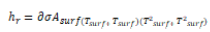 |
Table 1: Mode of heat transfer.
| Type of Micro Channel Heat Exchanger Tube | Pressure | Velocity |
|---|---|---|
| (In Pa) | (In M/S) | |
| Circular | 9 | 2 |
| Rectangular | 10 | 1 |
| Trapezoidal | 7 | 3 |
Table 2: Comparison of results based on CFD.
Conclusion
In the phase-I the domain, device and the existing analysis was identified. The geometry was developed starts with 2D sketching and finalized with 3D part modeling. An existing analysis had been done with the static structural analysis, thermal analysis for circular shape tube. As the results has planned to improve with the new proposed shapes like trapezoidal and rectangular tubes of heat exchanger. The design of the heat exchanger tube has modified with respect to new geometrical specifications. The material change has planned to modify from a trial with copper to nickel silver. Then an analysis proceed with static structural, thermal and computational fluid dynamics in phase-II and the results are gained. Apart from circular, rectangular and trapezoidal tube channels, the results are favor to trapezoidal tube, because of velocity outlet is greater than circular and rectangular tubes.
REFERENCES
- Drost K. Microscopic heat-actuated heat pump development. 1999.
- Erek A, Özerdem B, Bilir L, Ilken Z. Effect of geometrical parameters on heat transfer and pressure drop characteristics of plate fin and tube heat exchangers. Appl Therm Eng. 2005;25(14-15):2421-2431.
- Cao H. Optimization design of microchannel heat sink geometry for high power laser mirror. 2010.
- Barbosa JR. J Braz Soc Mech Sci Eng. 2010.
- Jang JY. Numerical experimental studies of three dimensional plate fin and tube heat exchanger. 1996.
- Bohn KM. Successful upscale of laboratory micro reactor into industrial scale. 2006.
- Kays WM. Compact heat exchangers. Krieger Publications. 1998.
- Malecha K. Microchannel fabrication process in LTCC ceramics. 2008.
- Mark E. Single phase liquid heat transfer in plain and enhanced micro channels. 2006.
- Martinez CS. LTCC microflow analyzers with monolithic integration of thermal control. 2007.
- Determan MD. Experimental demonstration of a microscale monolithic modular absorption heat pumps. 2012.
- Madou M, “Fundamentals of micro fabrications. 2002.
- Nag PK. Heat and mass transfer. Tata McGraw-Hill. 2006.Ffff
- Sachdeva RC. Fundamentals of engineering heat and mass transfer. New Age International Publications. 2012.
- Sachdeva RC. Fundamentals of engineering heat and mass transfer – Data Book. New Age International Publications. 2012.
- Seabra A. Monolithic continuous flow micro analyzer with amperimetric detection based on green technology. 2009.
- Taylor BN. Guidelines for evaluating and expressing the uncertainty of NIST measurement. 1994.
- Tonomura O. CFD Based optimal design of manifold in plate fin microdevices. 2004.
- Cengel YA. Heat and mass transfer: A practical approach. Tata McGraw Hill. 2007.
- Qu W. Analysis of three dimensional heat transfer in micro channel heat and mass transfer. 2002.
Citation: Balamurugan S (2021) Design and Analysis of Micro Channel Heat Exchanger with Different Geometry Configuration. J Appl Mech Eng. 10:394.
Copyright: © 2021 Balamurugan S. This is an open-access article distributed under the terms of the Creative Commons Attribution License, which permits unrestricted use, distribution, and reproduction in any medium, provided the original author and source are credited.