Indexed In
- Open J Gate
- RefSeek
- Hamdard University
- EBSCO A-Z
- OCLC- WorldCat
- Publons
- International Scientific Indexing
- Euro Pub
- Google Scholar
Useful Links
Share This Page
Journal Flyer

Open Access Journals
- Agri and Aquaculture
- Biochemistry
- Bioinformatics & Systems Biology
- Business & Management
- Chemistry
- Clinical Sciences
- Engineering
- Food & Nutrition
- General Science
- Genetics & Molecular Biology
- Immunology & Microbiology
- Medical Sciences
- Neuroscience & Psychology
- Nursing & Health Care
- Pharmaceutical Sciences
Research Article - (2023) Volume 12, Issue 3
Application of Temporal Sentinel 1 SAR Data for Multiple Crop Type Classification in a Command Area
Sobhan Mishra*, Annie Maria Issac, Syama S Rao, Ronald Singh, P V Raju and V V RaoReceived: 12-Mar-2020, Manuscript No. JGRS-23-3617; Editor assigned: 18-Mar-2020, Pre QC No. JGRS-23-3617(PQ); Reviewed: 01-Apr-2020, QC No. JGRS-23-3617; Revised: 24-May-2023, Manuscript No. JGRS-23-3617(R); Published: 21-Jun-2023, DOI: 10.35248/2469-4134.23.12.301
Abstract
Assessment of cropped area during kharif season is a difficult task due to the presence of cloud, cloud shadows and haze. So microwave datasets provide a good alternative as they have cloud penetration capacity. But deriving crop related information from microwave datasets is difficult task as it is subjected to different factors like phonological stage of the crop during satellite image acquisition, presence of speckle, polarization and the classifier used. In this study suitable filter polarization and classifier is identified by systematic analysis of time series, back scatter values derived from Sentinel 1 Synthetic Aperture Radar (SAR) data. As per the study, for the selected study area and time period, Sentinel 1-SAR images subjected to speckle removal by Intensity Driven Adaptive Filter (IDAN) filter proved to perform well in classification as against other filters. The time series of speckle removed VH polarization images classified using Random Forest classifier gave an accuracy of 45 percent in classifying paddy, nonpaddy and fallow.
Keywords
Speckle; IDAN filter; Polarization; Random forest classifier
Introduction
Mapping of major crop types with its spatial distribution is an important step for crop monitoring and yield estimation. The multispectral datasets for single and multiple dates from different satellite platforms were used in the identification of crop extent, its condition in different studies around the world. Cloud cover possesses a challenge on the availability of time series optical datasets which is very much necessary for the identification of crop types. In cloud cover conditions microwave datasets becomes very useful for monitoring crop types and its extent. Crop type information can be obtained from microwave datasets by using single scene or time series images. Time series datasets used to give a better degree of clarity for mapping out cropped areas. Temporal variation in backscatter coefficient (σ0) of Paddyfrom showing to vegetation is very predominant as paddy at the time of showing shows least backscatter due to ponded water and when the crop is established, it shows higher backscatter. The variation in the temporal trendsof backscatter values over Paddy, Non-Paddy and Fallow lands makes these three classes separable [1]. The back scatter obtained was correlated with crop age, its height and its biomass to identify different crop types. Microwave datasets are affected by speckle, which is corrected at the time of preprocessing. In order to extract information it becomes necessary to reduce speckle. Speckle is a salt pepper appearance that occurs due to interference between two waves reflected from scattering over terrain surface. Image filtering is a procedure in which the original pixel values are replaced with some values computed by using neighboring pixel values. There are two types of filter Non adaptive and adaptive filters. Non adaptive filter use same set of weights to smooth the entire image (Mean, median and mode) on the other hand adaptive filter use weights based on degree of speckle in the image (Lee, frost, Gamma, IDAN etc.). The image smoothing depends more on local statistics for adaptive filter, for which they preserve more details than non-adaptive filter.
Speckle corrected backscatter values generated from different polarization (HH, HV, VV and VH) exhibit similar temporal trends; the range of values over the same land cover varies depending on the polarization. It was found that time series backscatter values generated from HV polarization C band SAR images gave superior separabilityfor identifying crop types. Different studies were carried out by using different microwave frequencies with respect to biomass of the plant. The accuracy of in the identification of cropped area with its type from SAR datasets depends on polarization and frequencies.
Higher the frequency of microwave, lesser is the penetration power of microwave with respect to biomass and lower the frequencies higher the penetration of microwave with respect to biomass. Some studies were conducted in which multi frequencies (Ka, Ku, X, C, S and L) microwave datasets were used for identification of paddy fields and it was observed that L and S frequencies showed better correlation with respect to variation of biomass of crop [2]. With the advent of machine learning approaches the accuracy of classification of microwave images for obtaining crop type information had improved to a very high level. Classifying algorithms like maximum likelihood, gausian naive bayes, support vector machine, random forest, decision tree etc. are employed in satellite image classification along with training samples derived in conjunction with ground information.
This study aims for identification of suitable filters that can be used during preprocessing workflows for getting better distinction between major crop types and its spatial distribution. Importance was also given on selection of suitable machine learning classifier [3]. Sentinel 1 datasets were used for this purpose so importance was also given on selection of suitable polarization and dates for analysis purpose.
Materials and Methods
Study area
The Narayanpur irrigation system is a part of Krishna river basin, which falls in Gulbarga and Raichur district of Karnataka State as seen in Figure 1. It lies between 77°05’ to 76°77’ east longitude and 16°34’ to 16°6’ N latitude. The meteorology of the study area is, it experiences an annual precipitation of 711 mm and an annual average temperature of 27°centigrade. The maximum temperature in the region ranges from 39°centigrade and minimum temperature is about 22° centigrade. The system irrigates is expected to irrigate a maximum of 3,84,997 Ha [4]. The area has predominantly black cotton soil and red soil which is suitable for cultivation of paddy, cotton, legumes and millets.
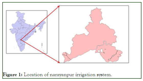
Figure 1: Location of narayanpur irrigation system.
Datasets used in the study
Satellite datasets: The Sentinel 1 SAR images for the months of June to November of the year 2018, having 12 days temporal frequency were used in the study. Sentinel 1-SAR provides datasets in two polarization VV (Vertical Send And Vertical receive) and VH (Vertical send and Horizontal receive), with a spatial resolution of 10 m. Mostly Ground Range Detection (GRD) datasets in Interferometry Wide swath (IW) mode products were used in the study.
During the period of June to November 2018 Sentinel 1-SAR datasets were acquired over Narayanpur irrigation system for 14 dates [5]. Of the 14 dates, 3 dates were selected for analysis based on thephonological development of the crop through the season. Datasets used for analysis are illustrated in Figure 2.
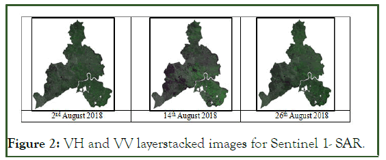
Figure 2: VH and VV layerstacked images for Sentinel 1- SAR.
Ancillary datasets : Ancillary datasets like command area boundaries digitized from high resolution datasets and sub basin boundaries obtained from terrain processing of digital elevation models were used in the study (India-WRIS).
Ground truth datasets:The training samples for classification was derived in conjunction with ground truth information collected by using hand held Global Positioning Devices (GPS) in Narayanpur irrigation system during 18th, 19th and 20th September 2018. In this process agricultural field was geo-tagged and crop related information like crop types, its irrigation source, stage of growth and its date of sowing information’s were collected [6]. Around 150 points were collected. Distribution of ground truth points throughout the study area is illustrated in Figure 3.
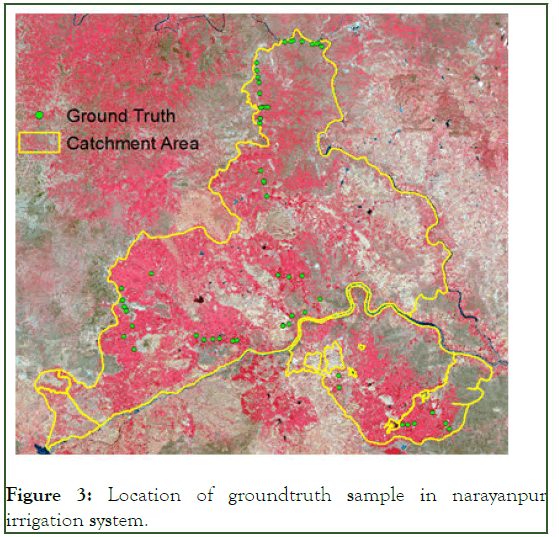
Figure 3: Location of groundtruth sample in narayanpur irrigation system.
The methodology for identification of paddy and non-paddy cultivated area from microwave datasets is illustrated in Figure 4. The steps involved are:
• Identification of suitable dates.
• Pre-processing of microwave datasets and identification of suitable filters.
• Identification of suitable polarization.
• Identification of suitable classifiers.
• Accuracy analysis by computing kappa statics.
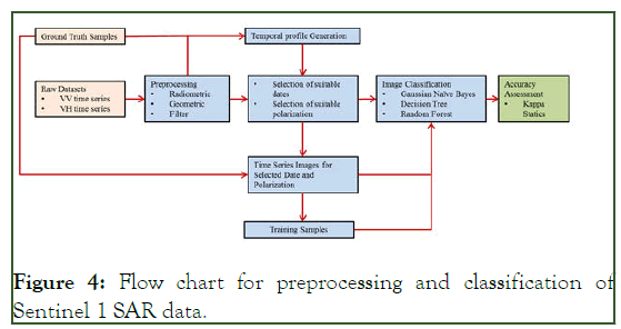
Figure 4: Flow chart for preprocessing and classification of Sentinel 1 SAR data.
Identification of suitable dates
Temporal backscatter values (σ0) profile was generated by using ground information collected, for both VH and VV polarization data for the datasets acquired during the period of June to November 2018. As observed in Figures 5 and 6 temporal backscatter coefficient profile for paddy, non-paddy and fallow profiles showed noticeable variations in the month of August [7]. Selecting the temporal backscatter values profile for entire season for paddy and non-paddy identification will complicate the analysis, Hence dates in month of August was selected.
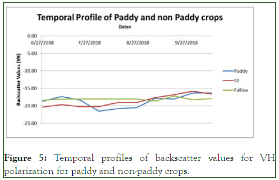
Figure 5: Temporal profiles of backscatter values for VH polarization for paddy and non-paddy crops.
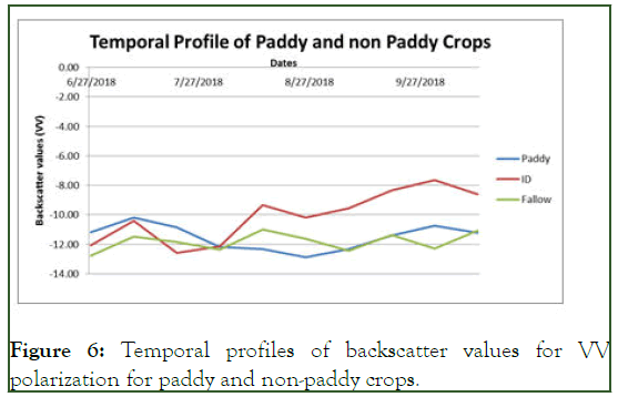
Figure 6: Temporal profiles of backscatter values for VV polarization for paddy and non-paddy crops.
Preprocessing of microwave datasets
Preprocessing of Sentinel 1 SAR datasets was done with help of SNAP toolbox. Radiometric, geometric and speckle filter was applied on the datasets to obtain backscatter values of individual dates for data sets in both the polarization [8]. In radiometric correction sigma naught backscatter values (σ0) were calculated.
Then geometric correction was carried out to avoid geometric distortions, which is caused due to geometry of sensor and shape of the objects. Filters are applied on the derived backscatter values for removal of speckles. There are many filters available for speckle removal. On application of filter, the distribution of the backscatter values is altered making the image smooth, removing the salt and pepper appearance.
There are different types of filter for removing speckle. The filters used in this study are boxcar, frost, gamma, median, lee sigma and IDAN. Boxcar averaging is a data treatment method that enhances the signal to noise of a signal by replacing the group of data points with its average. Frost Filter is an exponenti ally damped circularly symmetric filter that uses localstatistics [9]. The pixel being filtered is replaced with the value calculated based on the distance from the filter center, the damping factor and the local variance. Gamma filter is used to reduce speckle while preserving edges in radius image. The filter assumes that the data is gamma distributed and the pixel is replaced with value computed locally. Median filter smooth’s the image, while preserving edges larger than kernel dimensions. It replaces each center pixel with the median value within the neighborhood specified by the filter size. Lee sigma filter utilizes the statistical distribution of digital number values within the moving window to estimate the pixel of interest. It is based on the assumption that mean and variance of the pixel of interest is equal to the local mean and variance of all pixels within a selected moving window [10]. IDAN filter is Intensity driven adaptive neighborhood filter is atechnique in which the neighborhood is formed by using region growing technique driven exclusively by intensity image information.
The distribution of backscatter values in VV and VH polarization for a date was compared to understand the effect of different filters on the data. A time series layer stack of backscatter values in VV and VH polarization was subjected separability analysis to understand the suitability of filter for paddy, non- paddy and fallow area identification. The separability analysis was carried out to find out the degree of similarity and dissimilarity between the classes used for classification [11]. The seperability is quantified in terms of Transformed Divergence and Jeffries Matusita distance. Transformed Divergence gives an exponential decreasing weight for increasing distances between classes. Jeffries Matusita distance, is a function of Separability that directly relates to the probability of how good a resultant classification will be.
Identification of suitable polarization for classification of paddy, non-paddy and fallow land
Temporal backscatter profile for paddy, non-paddy and fallow classes was obtained from time series backscatter images in both VV and VH polarisation. Using 150 points for paddy, nonpaddy and fallow derived from the ground information, statistical parameters like mean, maximum, minimum, standard deviation and range was computed for all the three classes from both VV and VH data sets. Thepolarisation with least overlap among classes was selected for classification purpose.
Classification by machine learning algorithms
Three different machine learning approach was used for identification of paddy, non-paddy and fallow classesnamely gaussian naive bayes, decision tree and random forest.
Gaussian Naive Bayes employs Bayesian networks which are structures for representing the probabilistic relationship among large number of variables and doing probabilistic inference with that variable. This classifier mostly dealt with discrete variables, for continuous variable, a conditional Gaussian network paradigm is required without discretizing them [12]. The decision tree classifier is characterized by the fact that an unknown sample is classified into successive one or several decision trees for processing. There is a unique relationship between the string and the decision tree. The tree is encoded as a string of symbol such that there is an unique relationship between string and decision tree. The string is decoded in computer and points are set up to define appropriate classification path for each data sample. Random Forest classifier is an ensemble learning method for classification and regression that operates by constructing multiple decision trees at training time outputting the class that is mode of classes (classification) or mean prediction (regression) of individual trees. Random decision forest correct intermediate decision trees by over fitting their training sets.
Classification was done on time series VH backscatter image using the above discussed classifiers and accuracy of classification was assessed using Kappa statistics.
Results and Discussion
Selection of suitable filter
Statistical analysis: On application of filters the distribution of the backscatter values modified. The statistics of the backscatter values in VV and VH polarization is summarized in Table 1. As observed, on application of filters, standard deviation increased and the range of back scatter values decreased making the image more suitable for classification [13]. As illustrated in Figures 7 and 8, the IDAN reduced the range of backscatter values with higher standard deviation, making it best suitable filter with respect to statistical analysis.
| Filters | VH polarisation | VV polarisation | ||||||
|---|---|---|---|---|---|---|---|---|
| Min | Max | Mean | Std. dev | Min | Max | Mean | Std. dev | |
| No filter | -33.58 | 12.53 | -18.32 | 2.87 | -29.99 | 26.17 | -10.34 | 3.64 |
| Boxcar | -27.32 | 3.31 | -7.62 | 9.11 | -24.88 | 22.47 | -4.27 | 5.44 |
| Frost | -27.38 | 0 | -7.58 | 9.1 | -25.14 | 22.7 | -4.25 | 5.44 |
| Gamma | -27.34 | 7.205 | -7.58 | 9.1 | -25.56 | 21.45 | -4.25 | 5.43 |
| Lee sigma | -26.33 | 8.64 | -7.56 | 9.06 | -24.08 | 21.59 | -4.23 | 5.38 |
| Median | -27.79 | 0.23 | -7.6 | 9.13 | -25.49 | 22.09 | -4.28 | 5.47 |
| IDAN | -26.13 | 0 | -7.62 | 9.15 | -23.2 | 16.18 | -4.34 | 5.48 |
Table 1: Statistical range of backscatter values VH and VV polarization.
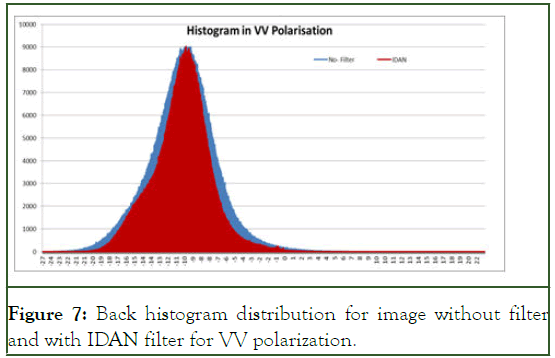
Figure 7: Back histogram distribution for image without filter and with IDAN filter for VV polarization.
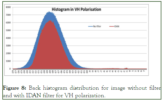
Figure 8: Back histogram distribution for image without filter and with IDAN filter for VH polarization.
Separability analysis: Separability analysis was carried out for the temporal back scatter profiles generated for the selected dates filtered by the six selected filters. The transformed divergence and jeffries-matusita distance was estimated and summarized in Table 2. It can be observed that the backscatter values derived from Intensity Driven Adaptive Filter (IDAN) filter was observed to give high separability values in both transformed divergence and jeffries matusita distance.
| Filters | Transformed divergence | Jeffries Matusita distance | |||||
|---|---|---|---|---|---|---|---|
| Paddy | Non-Paddy | Fallow | Paddy | Non-Paddy | Fallow | ||
| Boxcar | Paddy | 0 | 1553 | 1886 | 0 | 1206 | 1303 |
| Non-paddy | 1553 | 0 | 1902 | 1206 | 0 | 1336 | |
| Fallow | 1886 | 1902 | 0 | 1303 | 1336 | 0 | |
| Frost | Paddy | 0 | 1469 | 1862 | 0 | 1179 | 1265 |
| Non-paddy | 1469 | 0 | 1757 | 1179 | 0 | 1287 | |
| Fallow | 1862 | 1757 | 0 | 1265 | 1287 | 0 | |
| Gamma | Paddy | 0 | 1173 | 1418 | 0 | 710 | 1076 |
| Non-paddy | 1173 | 0 | 1558 | 710 | 0 | 1058 | |
| Fallow | 1418 | 1558 | 0 | 1076 | 1058 | 0 | |
| Lee sigma | Paddy | 0 | 1937 | 1501 | 0 | 1308 | 1197 |
| Non-paddy | 1937 | 0 | 1992 | 1308 | 0 | 1395 | |
| Fallow | 1501 | 1992 | 0 | 1197 | 1395 | 0 | |
| Median | Paddy | 0 | 1632 | 1017 | 0 | 1149 | 972 |
| Non-paddy | 1632 | 0 | 1866 | 1149 | 0 | 1272 | |
| Fallow | 1017 | 1866 | 0 | 972 | 1272 | 0 | |
| IDAN | Paddy | 0 | 1914 | 1995 | 0 | 1345 | 1387 |
| Non-paddy | 1914 | 0 | 2000 | 1345 | 0 | 1410 | |
| Fallow | 1995 | 2000 | 0 | 1387 | 1410 | 0 | |
Table 2: Seperability Values computed by transformed divergence and Jeffries Matusita distance for different filters.
Selection of suitable polarization for generation of time series backscatter values for classification
Box plot was generated for backscatter values of both VV and VH polarization for multiple dates selected as illustrated in Figures 9 and 10. It was observed that values in VH polarisation show lesser degree of overlap between paddy, non-paddy and fallow classes [14].
Hence, backscatter values in VH polarization was found better suited for classification as compared to back scatter values in VV polarization.
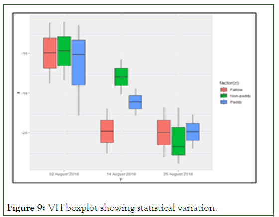
Figure 9: VH boxplot showing statistical variation.
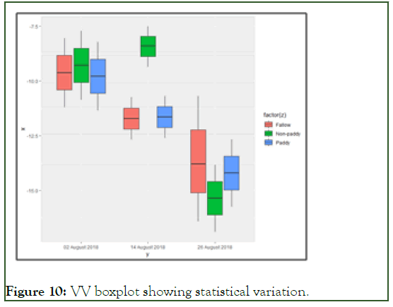
Figure 10: VV boxplot showing statistical variation.
Classification and accuracy assessment
Classification was carried out using three machine laerning algorithms namely random forest, gaussian naive bayes and decision Tree, on temporal back scatter profile in VH polarization subjected to IDAN filter. Training samples were generated from 10% of the ground truth points as illustrated in Figure 11. The crop maps generated are as seen in Figures 12-14. It was observed that the paddy area was over estimated by both Gaussian Naive Bayes and decision tree classifier.
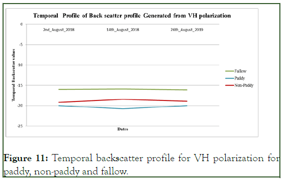
Figure 11: Temporal backscatter profile for VH polarization for paddy, non-paddy and fallow.
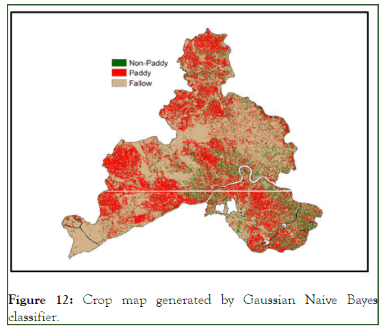
Figure 12: Crop map generated by Gaussian Naive Bayes classifier.
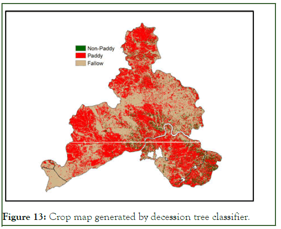
Figure 13: Crop map generated by decession tree classifier.
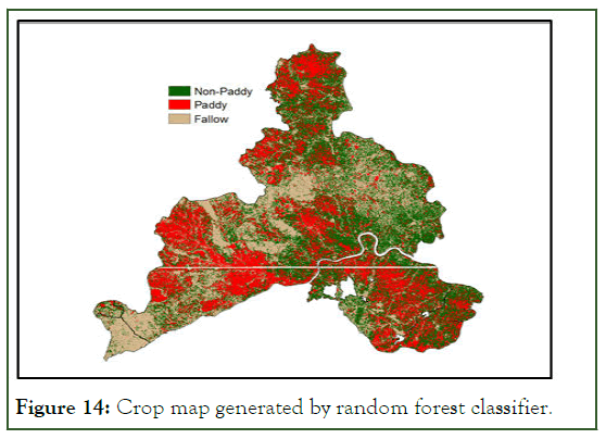
Figure 14: Crop map generated by random forest classifier.
The accuracy of classification was computed by estimation of Kappa statistics was computed for the maps generated from all the three classifier [15]. It was found that random forest classifier showed higher degree of classification accuracy with a Kappa value of 45 whereas Gaussian Naive Bayes and decision Tree gave a Kappa value of less than 25.
Conclusion
This study aimed for identification of suitable preprocessing methods and polarization of microwave data for identifying paddy, non-paddy and fallow areas using Sentinel 1 SAR datasets for Narayanpur irrigation system. Focus was given to identify cultivated lands within four weeks of sowing of paddy and non-paddy crops. Only sowing dates were taken into consideration for analysis in this study. Sowing dates gives a better discrimination between paddy, non-paddy and fallow. Intensity driven adaptive filter was found suitable as it showed higher degree of separability between paddy, non-paddy and fallow lands. VH polarized SAR data was best suited in this study area as the range of backscatter values showed minimum overlap among the classes. Random forest classifier proved to be best suited for classification of the temporal VH backscatter profiles for identification of the three classes under consideration. For identification of the paddy and nonpaddy classes, selection of dates during the sowing period in place of season time series will reduce the complexity in classification. Availability of adaptive fi lters for preprocessing and machine learning algorithms for classification can be best utilized for automated generation of crop maps from microwave datasets during Kharif season in absence of optical datasets.
References
- Al-Amri SS, Kalyankar NV, Khamitkar SD. A comparative study of removal noise from remote sensing image. Int J Comput Sci Issues. 2010;7(1).
- Apan A, Kelly R, Jensen T, Butler D, Strong W, Basnet B. Spectral discrimination and separability analysis of agricultural crops and soil attributes using ASTER imagery. IP R S Photogramm Conference (ARSPC 2002) 2002. University of Southern Queensland.
- Attema E, Snoeij P, Davidson M, Floury N, Levrini G, Rommen B, et al. The european gmes sentinel-1 radar mission. IEEE Int Geosci Remote Sens Symposium 2008;1:1-94.
- Attema EP. The active microwave instrument on-board the ERS-1 satellite. Proc IEEE. 1991;79(6):791-799.
- Attema EP, Ulaby FT. Vegetation modeled as a water cloud. Radio Sci. 1978;13(2):357-364.
- Becker-Reshef I, Justice C, Sullivan M, Vermote E, Tucker C, Anyamba A, et al. Monitoring global croplands with coarse resolution earth observations: The Global Agriculture Monitoring (GLAM) project. Remote Sens. 2010;2(6):1589-609.
- Brisco B, Brown RJ, Gairns JG, Snider B. Temporal ground-based scatterometer observations of crops in Western Canada. Can J Remote Sens. 1992;18(1):14-21.
- Dabboor M, Howell S, Shokr M, Yackel J. The Jeffries-Matusita distance for the case of complex Wishart distribution as a separability criterion for fully polarimetric SAR data. Int J Remote Sens. 2014;35(19):6859-6873.
- Douglas SC. Introduction to adaptive filters. Digit Signal Process. Boca Raton: CRC Press LLC. 1999.
- Du Y, Chang CI, Ren H, Chang CC, Jensen JO, D’Amico FM. New hyperspectral discrimination measure for spectral characterization. Opt Eng. 2004;43(8):1777-1786.
- Hastie T, Tibshirani R, Friedman JH, Friedman JH. The elements of statistical learning: Data mining, inference, and prediction. Springer Link, New York, 2009.
- Ho TK. Random decision forests. Int Conf Doc Anal Recognit. 1995;1:278-282.
- Inoue Y, Kurosu T, Maeno H, Uratsuka S, Kozu T, Dabrowska-Zielinska K, et al. Season-long daily measurements of multifrequency (Ka, Ku, X, C, and L) and full-polarization backscatter signatures over paddy rice field and their relationship with biological variables. Remote Sens Environ. 2002;81(2-3):194-204.
- Jia KU, Li Q, Tian Y, Wu B, Zhang F, Meng J. Crop classification using multi-configuration SAR data in the North China Plain. Intl J Remote Sens. 2012;33(1):170-183.
- Kussul N, Skakun S, Shelestov A, Lavreniuk M, Yailymov B, Kussul O. Regional scale crop mapping using multi-temporal satellite imagery. Int Arch Photogramm Remote Sens Spat Inform Sci. 2015.
Citation: Mishra S, Issac AM, Rao SS, Singh R, Raju PV, Rao VV (2023) Application of Temporal Sentinel 1 SAR Data for Multiple Crop Type Classification in a Command Area. J Remote Sens GIS. 12:301.
Copyright: © 2023 Mishra S, et al. This is an open-access article distributed under the terms of the Creative Commons Attribution License, which permits unrestricted use, distribution, and reproduction in any medium, provided the original author and source are credited.
