Journal of Remote Sensing & GIS

Accuracy Assessment of Spatial Interpolation Methods to Derives DEMs of Small Islands with Relative Topographic Variations

Hameid NA^1*, Bannari A², Kadhem G¹ and Abdelhadi AW^{3 1}Department of Geoinformatics, College of Graduate Studies, Arabian Gulf University, Manama, P.O. Box: 26671, Bahrain
²Space Pix-Map International Inc., #31 De-la-Clairière Street J8R-3R7, Gatineau (Québec), Canada
³Department of Natural Resources and Environment, College of Graduate Studies, Arabian Gulf University, Manama, Bahrain
^*Correspondence: Hameid NA, Department of Geoinformatics, College of Graduate Studies, Arabian Gulf University, Manama, Bahrain, Tel: +97336607137, Email:

Received: 15-Jun-2020 Published: 06-Jul-2020, DOI: 10.35248/2469-4134.20.9.275

Introduction

Digital Elevation Model (DEM) is a numerical representation of Earth surface topography. This model it is used to derive many topographic attributes in several geoscience applications (i.e., hydrology, geology, cartography, geomorphology, landslide, soil erosion, etc.), as well as performing geometric and radiometric corrections for topographic and shadow effects on remotely sensed imagery [1-4]. In combination with remote sensing and other geospatial data in a GIS environment, it can be used to model, simulate and/or visualize in 3D several natural resources, natural hazards and environmental phenomena (i.e., inundation, flash flood, Earthquake, wetlands discrimination, forest management, precision agriculture, etc.). Based on the requested accuracy and/or the nature of the project, which is often determined by economical aspects (investment vs. accuracy), as well as the conditions of surveying environment (e.g. terrain accessibility, topography and geometry, vegetation cover, etc.), DEM can be created by several methods. These include surveying engineering, stereo-photogrammetry, altimetric GPS in situ measurements, Lidar altimetry, radar interferometry (InSAR), topographic map contours, and stereoscopic pairs of optical satellite imageries, such as: SRTM (Shuttle Radar Topography Mission) and ASTER (Advanced Space borne Thermal Emission and Reflection Radiometer) [5,6]. However, independently to data acquisition mode, sometimes datasets contain gaps, irregularities and/or other anomalies that prevent immediate use in many applications. Nevertheless, these anomalies (or voids) can be filled using a range of interpolation algorithms in conjunction with other sources of elevation data [7].

Furthermore, it has been demonstrated that independently to the data acquisition method and the application, the DEM accuracy can vary to a certain degree with different interpolation algorithms [8]. Indeed, numerous mathematical models have been developed on spatial interpolation for topographic or bathymetric information densification. More than 40 spatial interpolation models and methods are described and classified into three different groups: deterministic, stochastic and combined methods [9]. These methods are mainly integrated in the emerging advanced geostatistical software technologies for users and specialists. For instance, most of them are accessible in ArcGIS [10] and other mapping software’s. Theoretically, the best and the most appropriate topographic surface interpolation method must reproduce the land terrain shape as closely as possible [11-14]. Nonetheless, the selection of an appropriate spatial interpolation method for small islands, DEM derivation is not an easy task [5]. As reported by many scientists, the performance of spatial interpolators depends on many factors [9], and it seems that there is no justification regarding the choice of an appropriate method because where each specifically is the “best” only for specific situation and application [15-18].

Likewise, small islands developing countries are characterized by small low-lying coastal zones, limited in size, and most vulnerable to the global warming and climate change impacts [5,19]. Moreover small island countries have vulnerable economies and depend both on very limited resource bases and on international trade, with limited means to influence the terms of that trade. Around the world, there are approximately 52 small islands developing countries among them 37 are identified as independent nations including the Kingdom of Bahrain [20]. The most environmental catastrophes experienced by these small islands are SLR, cyclones, volcanic eruptions, earthquakes, landslides, coastal inundation and erosion, and infrastructure destruction [21]. For instance, the lowlying nature of the coastal zones of Bahrain islands coupled with significant land reclamation investments and extensive industrial, commercial, and residential activity, emphasize the country’s critical vulnerability to SLR [22]. These will produce environmental, ecological and socio-economic sever impacts [23]. For instance, the increasing vulnerability due to coastal inundation may lead to considerable natural hazards, such as: the loss of coastal, damage to infrastructure, displacement of the population, loss of agricultural production, etc. [24]. Obviously, these negative natural disasters constitute severe and significant long-term menaces to small islands [25]. Consequently, several international organizations have pointed out the necessity to produce comprehensive impact assessments of SLR, especially on small islands, in order to establish scenarios or impact studies for proper adaptation and mitigation policies [26]. In these contexts, accurate DEM is the most appropriate for assessing the vulnerability of coastal zones vulnerability to SLR [27]. However, the quality and the accuracy of the used DEM in such environment are automatically related to the accuracy of the phenomenon under investigation, the source of input data, and the selected interpolation method [28]. To provide a clear idea and useful suggestions to scientists and decision maker, especially for SLR scenarios or hazards impact studies over Kingdom of Bahrain, the aim of this study is a comparison and assessment of absolute surface heights accuracies of derived DEMs based on deterministic (IDW, Spline, and Natural neighbour) and stochastic (Kriging) interpolation methods.

Materials and Methods

The methodology pathway applied is presented in Figure 1. Three deterministic methods were considered including the IDW with variable and fixed parameters, the Spline with regular and tension conditions, and the Natural Neighbor. While, for stochastic methods, the ordinary and simple Kriging were analyzed according to the semi-variogram adjustment considering five mathematical functions: Stable, Circular, Spherical, Exponential and Gaussian. The dataset input for the interpolation methods to derive the DEM’s was a very large scale topographic contour lines map (1:5000) generated from photogrammetric stereo-preparation and restitution exploiting optico-mechanic stereo-plotter and aerial photographs. For validation purposes, a datasets of 400 ground control points (GCPs) were used. They were uniformly distributed over the Bahrain territory in order to cover the existing altitude classes, and they were measured using Differential Global Position System (DGPS) with ± 1 cm and ± 2 cm for planimetric and altimetric accuracies, respectively.

Figure 1: Flowchart of the used methodology.

Study area

The Kingdom of Bahrain (26° 00’ N, 50° 33’ E) is anarchipelago located in the Arabian Gulf, east of Saudi Arabia and west of Qatar (Figure 2). The archipelago comprises 33 islands, with a total land area of about 800 km2 in 2017. Bahrain topography composed of five distinctive physiographic zones [4,29]. The first region is the coastal lowlands with elevation less than 10 m above mean sea level and slopes less than 0.5%. The second region is the upper Dammam back-slope which reflects the general asymmetrical shape of the main Bahrain dome whit elevation between 10 and 20 m, and slopes less than 5.4%. The third region is the multiple escarpment zones surrounding the interior basin of the island, it is a continuous belts of low multiple enfacing escarpments. From the north-west to the south-west of this region, the elevation and slopes varies significantly, respectively, from 20 to 34 m and from 5.4 to 14%. The fourth region is the interior basin which looks as an asymmetrical ring of lowlands surrounds the central plateau region (fifths region) whit relatively height elevation and strong slopes classes, respectively, 34 to 51 m and 14 to 29.5%. Finally, the fifth region is central plateau with upstanding residual hills and mountain. In this region, the elevations and slopes varies significantly between 51 and 134 m for JabalDukhan (the highest point in Bahrain) and 30 to 81%, respectively [30].

Figure 2: Study site location (Kingdom of Bahrain).

Interpolation methods

Spatial interpolation can be applied by deterministic (local), stochastic (global) or combined methods. In general, the process is based on the use of points with known attribute values to estimate the same attribute on other unknown points. The global method considers all the sampling points in the study area to make feature fitting for the study area [31]. While, the local method uses only the neighboring points to estimate the unknown point values [32,33]. However, estimations of nearly all spatial interpolation methods can be represented as weighted averages of sampled data. They all share the same general fundamental estimation Equation 1, which is the following [9]:

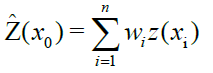
Where Ž is the estimated value of an attribute at the point of interest x₀, Z is the observed value at the sampled point x_i, w_i is the weight assigned to the sampled point “i”, and “n”represents the number of sampled points used for the estimation [34]. In the following paragraph, the interpolators employed in this work are briefly described.

IDW: The IDW is a local deterministic method based on autocorrelation concept. It estimates the value of an unknown attribute in a specific point using a linear combination of known attribute values weighted by an inverse function of the distance from the point under investigation to the known or observed points within a well-defined neighborhood. The selection of this neighborhood is based on the choice of a circle with varying size or a fixed number of known (observed) points, hence the names of variable or fixed IDW. It is based on the assumption that the known points closer to the unknown points are more similar than those further away in their values [1,35,36]. In other words, greater weights are given to points closest to the predicted locations, and the weights diminish as a function of distance. The main factor affecting the accuracy of IDW is the value of the power parameter [15]. The impact of the weights decrease as the distance increases between observed and estimated points, especially occur when the value of the power parameter increases. Consequently, nearby samples have a heavier weight and more influence on the estimation, where the power parameter and neighborhood size selection are arbitrary [9]. However, according to literature, the most popular choice of the power “p” is “2” and the method used is often inverse square distance or inverse distance squared [9,34]. The weights can be expressed in Equation 2 as:

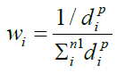
Where d_iis the distance between x₀ and x_i, p is a power parameter, and n represents the number of sampled points used for the estimation.

Spline: The Spline interpolation method estimates unknown attribute values almost similarly to IDW but with some specific conditions according to the integrated mathematical function in the adjustment and estimation process [35-38]. Indeed, Spline method include different mathematical function types that minimizes overall surface curvature, resulting in a smooth surface that passes exactly through the input points. These functions are the Thin-plate, the Multi-quadric, the Inverse Multi-quadric, the Tension and the Regularized function [39,40]. Only the latter two functions are considered in this study. The Regularized function creates a smooth, gradually changing surface with values that may lie outside the sample data range. Whereas, the Tension function controls the abrupt change of the surface according to the character of the modeled phenomenon. It creates a less smooth surface with values more closely constrained by the number of input sample data. Indeed, for the both selected methods the output surface is accomplished through two fundamental parameters: weight and number of known sampling points. For Regularized method, the weighted parameter defines the weight of the third derivatives of the surface in the curvature minimization expression. Obviously, the higher the weight, the smoother the output surface. In ArcGIS environment, the typical values entered for this parameter are 0, 0.001, 0.01, 0.1, and 0.5,whereas, in the Tension method, the weight defines the tension power. The typical values to be introduced in ArcGIS must be equal to or greater than zero (i.e., 0, 1, 5, and 10). According to many applications, the higher the weight, the coarser will be the output surface. Furthermore, regarding the number of known sampling points introduced as an input to the interpolation process, usually that more input points are considered, the more each estimated point will be influenced by distant points and the smoother the output surface will be. According to ESRI (2015), these methods are best for generating slightly varying surfaces such as elevation, water table heights, or pollution concentrations.

Natural neighbors: This method has been introduced by Sibson, which, also known as Sibson or “area-stealing” interpolation. This method combines the concepts of two unlike process: nearest neighbors and triangular irregular network (TIN). In two interrelated steps, this method finds the closest subset of input samples to a query point and applies weights based on proportional areas in order to interpolate the value of unknown point. The first step is a data triangulation following the Delauney’s method, wherein the vertices of the triangles are the sample points in adjacent Thiessen polygons. The second step is to estimate the value of an unknown point, where it is inserted into the tessellation and then its value is determined by sample points within its bounding polygons [34,41]. In other words, its basic properties are local, using only a subset of samples that surround a query point, and that interpolated heights are guaranteed to be within the range of the samples used. On the other hand will not infer trends and, will not also produce peaks, pits, ridges or valleys that are not already represented by the input samples. Moreover, this method passes through the input samples and smooth everywhere except at locations of the input samples. Break-lines may be used in the TIN process to create linear discontinuities where appropriate, such as: along roadsides and water bodies. It adapts locally to the structure of the input data, requiring no input from the user pertaining to search radius, sample count, or shape, and it works equally well with regularly and irregularly distributed data [40].

Kriging: Kriging is a global stochastic or geostatistical interpolation method that considers both the distance and the degree of variation between known attribute points to estimate attribute values of unknown points. It works similarly to IDW method [41] with exception of the weights which are not based only on the distance between the known and unknown points but on the overall spatial arrangement of the known points. Kriging assumes that the distance or direction between sample points reflects a spatial correlation that can be used to explain the variation in the surface [31]. It is a multistep analysis process that fits a mathematical function to a specified number of points, or all points within a specified radius, to determine the output value for each location using sophisticated weighted average technique [42]. Indeed, it derives the spatial arrangement in the weights by quantifying the spatial autocorrelation using the semi-variogram based on one of the following mathematical functions: circular, spherical, exponential, Gaussian and linear [35,43]. There are two kriging methods; ordinary and simple. The ordinary kriging (OK) assumes that the constant mean is unknown, on the other hand the simple kriging (SK) assumes that there is a dominant trend in the data and this trend can be modeled by a polynomial function. Kriging fits a mathematical function to a specified number of points, or all points within a fixed radius, to determine the output value for each unknown point [9].

The semi-variance (γ) of unknown point Z between two known data points (one pair of sample points) is an important concept in geostatistics (Equation 3), as well it can be estimated from “n” pairs of sample points as indicated in Equation 4, as follow:

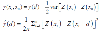
Where “d” is the distance between points x₀ and x_i, and γ (d) is the semi-variogram, as well commonly referred as variogram [34]; while “n” is the number of pairs of sample points separated by distance “d” [11]. The semi-variogram modeling, analysis and estimation are extremely important for structural analysis and spatial interpolation based on the input of: nugget, range and sill. The “nugget” is a residual reflecting the variance of sampling errors and the spatial variance at a shorter distance than the minimum sample spacing. The “range” is a value of distance at which the “sill” is reached, providing information about the size of a search window used in the spatial interpolation methods. Samples separated by a distance larger than the range are spatially independent because the estimated semivariance of differences will be invariant with sample separation distance. If the ratio of “sill” to “nugget” is close to 1, then most of the variability is attributed to non-spatial [44].

Accuracy assessment

The accuracy of DEMs derived from different and independent interpolation methods was assessed by reference to elevation data acquired with DGPS representing the elevation truth. According to the American Society for Photogrammetry and Remote Sensing [45], the elevation accuracy of each DEM should be expressed by the root mean square error (RMSE) given by the following Equation 5:

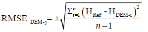
Where HRef is the reference DGPS elevation data (in situ measurements), HDEM-i is the elevation derived from the used interpolation method, and “n” corresponds to the total number of DGPS GCPs used for validation. As recommended by USGS (1997), DEM accuracy assessment is usually made with a minimum of 28 GCPs. However, Li reported that many GCPs are needed to achieve a consistency closer to what is accepted in most statistical tests. Indeed, the number of the used GCPs for validation is an important factor in consistency because it adjusted the range of stochastic variations on the RMSE and standard deviation values [46]. In this study, 400 GCP points were used for accuracy assessment, measured with DGPS assuring accuracies of ± 1 and ± 2 cm for planimetry and altimetry, respectively. These points were uniformly distributed over the study area considering all existents topographic terrain variability’s (different slopes, orientations, elevations, roughness, etc.).

Results and Discussion

The accuracy assessment of the derived DEMs based on the considered interpolation methods is a critical step for information extraction analysis. In addition to statistical methods that are often used for DEMs exactitudes analysis, visual interpretation methods are generally important for derived thematic maps quality assessment. Certainly, the complementarily between these two methods of analysis (visual and statistic) would result in a more efficient improvement of the derived product quality.

Visual analysis

In order to have a reliable comparison reference, it is necessary to describe the topographic classes of the study area accurately according to geodesy and surveying engineering methods. Generally, the topography of Bahrain has low variability with five major physiographic regions (4,30,31). The first region is the coastal lowlands, with an elevation of less than 10 m above mean sea level characterized with slopes less than 0.5%. The second region is the upper Dammam back-slope reflecting the general asymmetrical shape of the main Bahrain dome with elevations that vary between 10 and 20 m, and slopes less than 5.4%. The third region is the multiple escarpment zones surrounding the interior basin of the island. From the northwest to the southwest of this region, elevations and slopes vary significantly from 20 to 34 m and from 5.4% to 14% respectively. The fourth region is the interior basin, which appears as an asymmetrical ring of lowlands surrounding the central plateau (fifth region) with relatively higher elevations (34 to 51 m) and steeper slope classes (14% to 29.5%). The central plateau (fifth region) has upstanding residual hills and a more mountainous-type terrain, with greater variations in elevation (51 to 134 m) and slopes (30% to 81%) and includes Jabal-Dukhan (the highest point in Bahrain, i.e. 134 m). According to this topographic description, it is possible to distinguish among four major groups of drainage (catchments) zones that mimic the major physiographic areas: the coastal lowland, the upper Dammam backslope, the multiple escarpment zones, and the interior-basin and central plateau.

Furthermore, two derived DEMs were generated based on IDW methods, characterized byvariable and fixed parameters. For the first method, after many tests, the optimal results were obtained using a number of 12known points that are the nearest to the unknown and estimated points. While, the second method adopted a fix radius at 20 mand all known points within this radius were considered in interpolation process. Figures 3a and 3b illustrate the derived DEMs using both methods;thus the output cell was setto 2.5 m.In general, the tow generated DEM reflect the five major topographic classes. However, the IDW method with variable parameters smooth the terrain texture, roughness and the micro-topography; and change the output values of the introduced low and high altitudes (Figure 3a). Indeed, the very low altitude at the mean sea level (MSL) which is null value (zero) was estimated to +1.87 m, whereas the highest altitude was overestimated with +0.50 m. While, the derived DEM based on IDW with fixed parameters reflect correctly the five topographic classes describing properly the geomorphological variability without smoothing or change in micro-topography of terrain roughness. It conserve the integrity of the original value of low altitude at the MSL, but it overestimate the high altitude at Jabal-Dukhan with +0.20 m (Figure 3b).

Figure 3: a) Derived DEM using IDW with variable parameters; b) Derived DEM using IDW with Fixed parameters.

Figures 4a and 4b illustrate obtained DEMs maps applying regularized and tension spline methods. These results revealed that the morphology of the original five topographic classes has not been characterized in both methods and are not relevantfor Small-Island topographic attributes derivations. Indeed, the both methods smoothed the abrupt topographic variations producing important fuzzy aspects of topographic classes and fragment the uniform and flat terrains of lowland class.Moreover, the regularized method generate a maximum elevation of +237.3 m for Jabal-Dukhan (i.e. overestimation with +103 m) and a minimum elevation of -123 m by reference to MSL that must be zero (Figure 4a). Thereby, the tension method estimated the minimum and the maximum altitudes to -65m and +130 m, respectively (Figure 4b). By reference to the original data introduced in the interpolation process we observe that the predicted altitude of Jabal-Dukhan was underestimated with 4 m, and the MSL was underestimated with 65 m. These significant biases introduced by these two methods do not give them the possibility of being suitably used for the estimation and mapping of altitudes in small islands.

Figure 4: a) Derived DEM using Spline with regularized parameters; b) Derived DEM using Spline with tension parameters.

Otherwise, the Natural Neighbors method generate a smooth DEM, gradually changing topographic surfaces with values range between 0.00 and 134.3 m, which reflect correctly the lowest and the highest elevation points in Bahrain Island (Figure 5). Except the locations of the input samples with known values, this method smoothed all other areas of estimated altitude values. Moreover, it fails to describe correctly and independently the fourth topographic class (interior basin) with relatively higher elevations (34 to 51 m) and the fifth class (central plateau) with greater variations in elevation (51 to 134 m). Consequently, the topographic areas in Bahrain cannot be properly and accurately mapped with this method.

Figure 5: Derived DEM using Natural Neighbors method.

Figure 6: a) Derived DEM using S.K. with Exp. Function; b) Derived DEM using O.K. with Exp. Function.

Due to specific shape of Bahrain Island topography, ordinary and simple kriging interpolations were implemented considering several semi-variogram adjustments, based on the five mathematical functions (stable, circular, spherical, exponential, and Gaussian),and assuming a multiplicative skewing distributions. All combinations of tests were implemented, examined and adjusted until the best fit of the model was achieved. Finally, the interpolation procedure was carried out considering the contour lines, using eight (8) neighbor points, the direction trend analysis, the number of lags was fixed at 12, the lag size was 0.086, and the output pixel size was fixed to 2.5 m × 2.5 m. Among all tested cases, SK and OK based on the exponential function provided the best results as illustrated by Figures 6a and 6b.Visually the derived map are similar faithfully representing the five different topographic classes. They describe similarly the terrain shapes, forms, texture, roughness and micro-topography. By reference to the original data introduced in the interpolation process we observe that the altitude of Jabal- Dukhan was predicted at 134.40 m by the both methods, with an overestimation of +0.40 m. While, the lowest elevation at the MSL was estimated at +0.14 m and +0.22 m by SK and OK, respectively (Figures 6a and 6b). Comparatively to the deterministic methods, these very low biases are introduced because the Kriging method considered the spatial autocorrelation structure of elevations among the considered points.

Statistical Analysis

The relationships between the measured and estimated altitudes values were analyzed using a linear regression model (p<0.05). For the validation process, 400G CPs were measured using correlation DGPS and their homologous estimated from the DEMs based on the considered interpolation methods were compared using the 1:1 line. Ideally, the observed and predicted values should have a correspondence of 1:1. For the IDW variable parameters, the validation DGPS-GCPs showed fitness of (R2=0.93) with their homologous (Figure 7). The scatter-plot for this method show a good fit with 1:1 line with an intercept and origin of 0.96 and 0.68, respectively. However, although this good statistical fits, the yielded RMSE was found to be ± 3.73 m corroborating the visual interpretation results. Definitely, this method is not accurate enough to be applied for Small Island DEM derivation under SLR scenario simulations or any other application that requires accurate topographic information. While, the scatter-plot of IDW fixed parameters indicated that this method perform slightly better than the variable parameters. Indeed, this slight performance depicted the distribution of validation points around the fitting axis (1:1 line) expressing R2 of 0.99 with a slope of 0.98 (near to the unity) and intercept of 0.25. Unfortunately, the calculated RMSE was ± 1.94 m, which is also not sufficient for DEM use in several geoscience applications. In general, regarding these two methods, the statistical results are in agreement with those of visual interpretation.

Figure 7: Scatter-plot of DGPS-GCPs for validation and, homologous points indifferent DEMs based interpolation methods.

Furthermore, the validation scatter-plot obtained for regularized spline method (Figure 7) revealed some irregularity in the why that this method process the very high and very low altitudes. Indeed, the low altitudes are significantly underestimated and oppositely the high altitudes are strongly overestimated. The distribution of validation points around the fitting axis (1:1 line) are not well fitted showing an R2 of 0.51. As well as the slope (1.31) and intercept (-8.38) are supporting this low fit, yielding a very strong RMSE of ± 24.36 m. Although the results of spline tension interpolation revealed a better adjustments than the regularized method, especially for moderate and high altitudes, the lowest altitudes are significantly underestimated. In fact, the presented scatter-plot in the Figure 7 exhibited an R2 of 0.77 with a slope of 1.04 and intercept of -2.95. Whereas, the calculated RMSE is approximately ± 10.60 m, which is not consistent with accurate topographic attributes integration in many DEM applications. Otherwise, the scatter-plot of Natural neighbors indicates that the results are inbetween the IDW variables and fixed parameters methods with R2 of 0.96, slop of 0.97, and the intercept of 0.03. Nevertheless, the resulting RMSE is equal to ± 3.87 m, expressing a large variability of altitudes difference. Obviously, due to specific shape of Bahrain island topography, this accuracy is not adequate for SLR scenarios or any other hydrological application. Finally, for simple and ordinary Kriging, the estimated altitude values based on these two methods showed high fitness (R2=0.96) with their homologous. These scatter-plots illustrate in general a good fit to 1:1 line with a slop of 0.96 (near to unity) and an intercept of 0.36. Moreover, these methods exhibit the best RMSE of ± 0.65 m that is less than the tolerance or the total calculated error (± 0.78 m)based on errors sources propagation [47]. Consequently, the kriging approach is a powerful statistical interpolation method, adjusting to the spatial data structure and provided better estimations of the altitude than the other interpolation methods. Definitely, the derived DEM based on Kriging is more accurate for small island applications such as the evaluation of coastal zones vulnerability to SLR, flooding and the detection of topographic features and the magnitude of hydrological processes [48].

Conclusions

The aim of this research is a comparison of absolute DEM surface heights accuracies retrieval based on three deterministic interpolation methods, such asIDW with variable and fixed parameters, Spline with regular and tension conditions, and the Natural Neighbor. As well as, two stochastic methods (ordinary and simple Kriging) were considered applying the semi-variogram adjustment and analysis based on five mathematical functions, which are Stable, Circular, Spherical, Exponential and Gaussian. To achieve this objective, a very large scale topographic contour lines map (1:5000) generated from photogrammetric stereo-preparation and restitution exploiting optico-mechanic stereo-plotter and aerial photographs was used as input in the interpolation process. Likewise, for validation purposes, a datasets of 400 GCPs were used. They were uniformly distributed over the Bahrain territory in order to cover the existing altitude classes, and they were measured using DGPS with ± 1 cm and ± 2 cm for planimetric and altimetric accuracies, respectively. The results obtained show that visual interpretation and statistical analysis converge toward the same conclusions. The Spline methods are not able to identify adequately change in topographic attributes, achieving a very large RMSE of ± 24.36 m and ± 10.60 m for regularized and tension process, respectively. Nevertheless, the IDW methods provides an RMSE of ± 3.73 m and ± 1.94 m for the variable and fixed parameters, respectively. Otherwise, the Natural neighbours method yield an RMSE of ± 3.87 m, expressing a large altitudes difference with the filed truth. Definitely, these deterministic methods revealed some irregularity in the way that they process the very high and very low elevations. Consequently, they are not accurate enough to be applied for Small Island DEM derivation under SLR scenario simulations or any other application that requires accurate topographic information. Contrariwise, the estimated DEM altitude values based on stochastic methods (simple and ordinary Kriging) fits similarly and very significantly (R2=0.96) with their homologous GPS’s measured with DGPS. They exhibited the best RMSE (± 0.65 m) which is less than the tolerance (± 0.78 m) which is the total altimetric error. Decidedly, the derived DEM based on Kriging is more accurate and adequately depicting the five major topographic classes in the study area, and identified the change in topographic attributes, shapes, forms and micro-topography. These two methods are more appropriate for small island applications such as the evaluation of coastal zones, vulnerability to SLR, flooding, detection of topographic features, and magnitude of hydrological processes.

Acknowledgements

The authors would like to thank the Arabian GulfUniversity for their financial support. We would like tothank the Surveyand Land Registration Bureau, Topographic surveyDirectorate (Kingdom of Bahrain) for the topographiccontour lines map and DGPS data. Finally, we express gratitude to theanonymous reviewers for their constructive comments.

REFERENCES

1. Burrough PA, Principles of Geographic Information Systems. 1st edn. Oxford University Press, New York, 1986;336.
2. Lee J. A drop heuristic conversion method for extracting irregular networks for digital elevation models. Proceedings of GIS/LIS '89, Orlando, U.S.A. 1989;30-39.
3. Bannari A, Morin D, Bénié GB, Bonn F. A theoretical review of different mathematical models of geometric corrections applied to remote sensing images. Rem Sens Rev. 1995;13:27-47.
4. Bannari A, Kadhem G, El-Battay A, Hameid NA, Rouai M. Detection of areas associated with flash floods and erosion caused by rainfall storm using topographic attributes, hydrologic indices, and GIS. Rem Sens Rev. 2017;21:209.
5. Bannari A, Kadhem G, Hameid NA. El-Battay A. Small Islands DEMs and topographic attributes analysis: A comparative study among SRTM-V4.1, ASTER-V2.1, high topographic contours Map and DGPS. J Earth Sci and Eng. 2017;7:90-119.
6. Bannari A, Kadhem G, El-Battay A, Hameid N. Comparison of SRTM-V4.1 and ASTER-V2.1 for accurate topographic attributes and hydrologic indices extraction in flooded areas. J Earth Sci and Eng. 2018;8:8-30.
7. Reuter HI, Nelson A, Jarvis A. An evaluation of void-filling interpolation methods for SRTM data. Intern J GIS. 2007;21(9):983-1008.
8. Weng Q. Comparative assessment of spatial interpolation accuracy of elevation data. In Proceedings of 1998 ACSM Annual Convention and Exhibition, Baltimore, Maryland, USA. 1998.
9. Li J, Heap AD. A review of spatial interpolation methods for environmental scientists. Geoscience Aust Rec. 2008;23:137.
10. Law M, Collins A. ESRI Getting to Know ArcGIS, 4th edn. New York, USA. 2017.
11. Burrough PA, McDonnell RA. Principles of Geographical Information Systems. Oxford University Press, New York, USA. 1998;333-335.
12. Robinson TP, Metternicht GI. Comparing the performance of techniques to improve the quality of yield maps. Agri Sys. 2005;85:19-41.
13. Fencik R, Vajsablova M. Parameters of interpolation methods of creation of digital model of landscape. Conf GIS. 2006;20:374-381.
14. Yilmaz HM. The effect of interpolation methods in surface definition: An experimental study. Earth Surf Proc and Landforms. 2007;32(9):1346-1361.
15. Isaaks M, Srivastava RM. An Introduction to Applied Geostatistics. Oxford University Press: New York, USA. 1989.
16. Zimmerman C, Pavlik A, Ruggles A, Armstrong M. An experimental comparison of ordinary and universal Kriging and inverse distance weighting. Math Geology. 1999;31:375-390.
17. Priyakant N, Kiran VI, Rao M, Singh AN. Surface approximation of point data using different interpolation techniques, a GIS approach. Geospatial Research. 2003;22:118-122.
18. Hofierka J, Cebecauer T, Suri M. Optimization of interpolation parameters using a cross-validation. Best practice in digital terrain modelling: Development and applications in a policy support environment. Europ Comm J Res. 2005;12:13-19.
19. UN. United Nations Report of the Global Conference on the Sustainable Development of Small Island Developing States. Global Conference on the Sustainable Development of Small Island Developing States. 1994;22:1-77.
20. Singh D. Small Island Developing States SIDS: Tourism and Economic Development. Tourism Anal. 2008;13(5):629-36.
21. UNISDR, (United Nations Office for Disaster Risk Reduction). (2009). Global assessment report on disaster risk reduction. 2019.
22. Mclean RF, Tsyban A, Burkett V, Codignotto J, Forbes D. Climate change 2001: Impacts, Adaptation and Vulnerability. Cambridge University Press, Cambridge, UK. 2001;343-379.
23. Michael J, Episodic flooding and the cost of sea-level rise. Ecol Econ. 2007;63:149-159.
24. Titus G, Anderson E, Cahoon D, Gesch D, Gill S, Gutierrez B, et al. Coastal Sensitivity to Sea-Level Rise: A Focus on the Mid-Atlantic Region. Synthesis and Assessment Product 4.1 Report by the U.S. Climate Sci Global Change Res. 2009;7:12-20.
25. Sim R. Assessing the impacts of sea level rise in the Caribbean using geographic information systems. Ecol Econ. 2011;63:149-159.
26. UNEP (United Nations Environmental Programme) Status and Threats of, and Major Threats to, Island Biodiversity. Puerto de la Cruz, Canary Islands, Spain, UNEP. 2004.
27. Weiss JL, Overpeck JT, Strauss B. Implications of recent sea level rise science for low-elevation areas in coastal cities of the conterminous USA. Climatic Change. 2011;105:635-645.
28. Overpeck JT, Weiss J. Projections of future sea level becoming direr. Proc of Nat Acad of Sci USA. 2009;11:133-139.
29. Doornkamp JC, Brunsden D, Jones DKC. Geology, Geomorphology and Pedology of Bahrain. Geo Abstracts, Norwich, U.K. 1980.
30. Hameid NA, Bannari A, Ghadeer A. Absolute surface elevations accuracies assessment of different DEMs using ground truth data over Kingdom of Bahrain. J of Remote Sens. 2016;5(3):1-5.
31. Longley PA, Goodchild M, Maguire DJ, Rhind DW. Geographic Information Systems and Science. Earth Surface Processes and Landforms. 2010;22:526.
32. McCoy J, Johnston K. Using Arc Gis Spatial Analyst. Env Sys Res. 2002;11:32-42.
33. Wong DW, Yuan L, Perlin SA. Comparison of spatial interpolation methods for the estimation of air quality data. J Exp Sci and Env Epidemiol. 2004;14:404-415.
34. Webster R, Oliver MA. Geostatistics for environmental scientists. Env Eco Germ. 2001;13:117-126.
35. Liu H. Development of an Antarctic digital elevation model: Columbus, Ohio. Byrd Polar Res. 1999;19:157.
36. Tomeczak M. Spatial interpolation and its uncertainty using automated anisotropic inverse distance weghing (IDW),Cross-validation Jacknife Approach in Mapping radioactivity in environment. In: Dubois. Env Res. 2003;14:51-62.
37. Johnston K, VerHoef J, Krivoruchko K, Neil L. Using ArcGIS geostatistical analyst. Env Sys Res. 2001;15:222-225.
38. Franke R. Smooth interpolation of scattered data by local thin plate splines. Comp and Math App. 1982;8(4):273-281.
39. Desmet PJ. Effects of interpolation errors on the analysis of DEMs. Earth Surface Processes and Landforms. 1997;22:563-580.
40. Watson D. Contouring: A Guide to the Analysis and Display of Spatial Data, Pergamon Press, London, 1992.
41. Oliver MA. Kriging: A method of interpolation for geographical information systems. Intern J Geographic Information Systems. 1990;4:313-332.
42. Tan Q, Xu X. Comparative analysis of spatial interpolation methods: An experimental study. Sens Trans. 2014;165(2):155-163.
43. Pebesma EJ. Multivariable geostatistics in S: the gstat package. Comp and Geosci. 2004;30:683-691.
44. Hartkamp AD, De Beurs K, Stein A, White JW. Interpolation Techniques for Climate Variables. NRG-GIS Mexico. Sens Trans. 1999;11:221-250.
45. ASPRS, (American Society for Photogrammetry and Remote Sensing), ASPRS Accuracy Standards for Large-Scale Maps. Photogramm Eng and Rem Sens. 1990;56(7):1068-1070.
46. Li Z. Effects of Check Point on the Reliability of DTM Accuracy Estimates Obtained from experimental test. Photogramm Eng and Rem Sens. 1991;57:1333-1340.
47. Bannari A, Kadhem G. MBES-CARIS Data validation for bathymetric mapping of shallow water in the Kingdom of Bahrain on the Arabian Gulf. Remote Sens. 2017;9:385-404.
48. Sibson R. A Brief Description of Natural Neighbor Interpolation, in Interpolating multivariate data. John Wiley and Sons, New York, USA. 1981;12:21-36.